Write in front

Because I'm really lazy, and I don't have a solid basic knowledge of machine learning and deep learning, but I want to make some fun models under the banner of artificial intelligence. I heard here that a module can simply build a deep learning model, and the effect of adjusting the parameters is relatively good. What can I do because there are no tutorials on the Internet, Read and write by yourself.
Reference link:
GitHub source address: https://github.com/awslabs/autogluon
Official website tutorial: https://auto.gluon.ai/stable/index.html

install

At present, the module is only applicable to Linux and Mac systems, and the windows module is under development. If you want to have a taste, you can install wsl in windows, and then use the following statement to install the module

python3 -m pip install -U pip
python3 -m pip install -U setuptools wheel
python3 -m pip install autogluon
# cpu version
python3 -m pip install -U "mxnet<2.0.0"
# gpu version
# Here we assume CUDA 10.1 is installed.  You should change the number
# according to your own CUDA version (e.g. mxnet_cu100 for CUDA 10.0).
python3 -m pip install -U "mxnet_cu101<2.0.0"

Library function

In fact, the tasks to be completed in this library are divided into several tutorials, namely table prediction, image prediction, target detection, text prediction, etc. This article first completes the first tutorial table prediction

Tabular Prediction

Definition: according to personal understanding, this table prediction should belong to the input data table, and then do relevant machine learning tasks according to this information.
Advantages: no data cleaning, feature engineering, hyperparametric optimization and model selection

Example 1

Objective: to predict whether a person's income exceeds $50000

Import data, build objects

# import data 
import pandas 
import numpy 
from autogluon.tabular import TabularDataset, TabularPredictor
train_data = TabularDataset('https://autogluon.s3.amazonaws.com/datasets/Inc/train.csv')
subsample_size = 500  # subsample subset of data for faster demo, try setting this to much larger values
train_data = train_data.sample(n=subsample_size, random_state=0)
train_data.head()

The AutoGluon Dataset object constructed here, that is, TabularDataset, is the data equivalent to pandas Frame, so you can use pandas Use dataframe attribute to use it, such as train mentioned above_ data. head(). Similarly, if you have your own data, you can construct objects according to the following picture tips

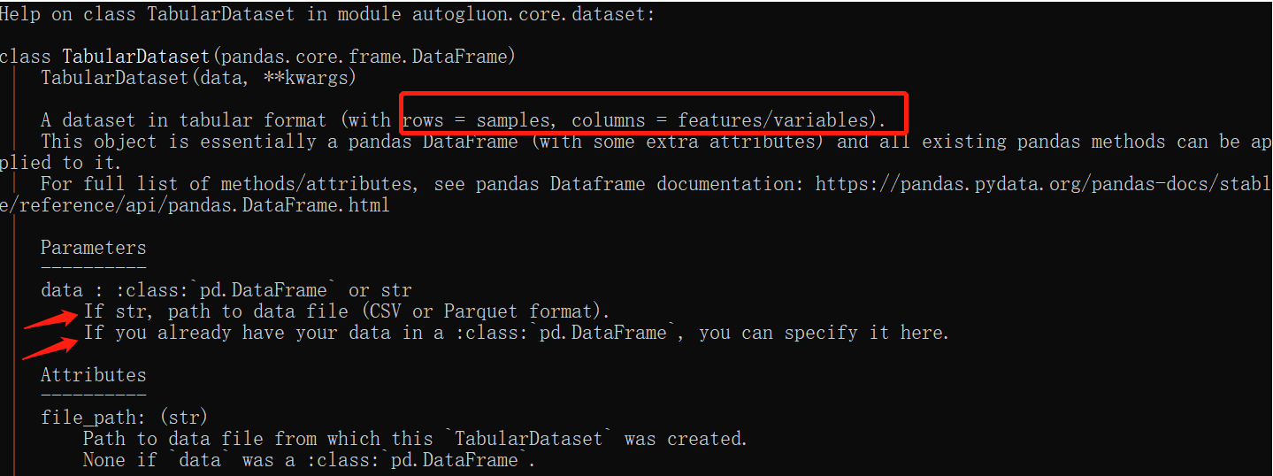
Anyway, check the help file when everything is in doubt

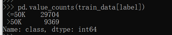
label = 'class'
pd.value_counts(train_data[label]) # Or train_data[label].value_counts() 
# The above two methods depend on personal habits
# Look at the labels and the number of corresponding labels

Training model

save_path = 'agModels-predictClass'  # specifies folder to store trained models
predictor = TabularPredictor(label=label, path=save_path).fit(train_data)

save_path is used to specify the folder of the training model
Then the TabularPredictor is used to build the model directly

The above figure is very interesting, which roughly explains why inference is a secondary classification task, how to modify it if it is not allowed, and how much memory is available now

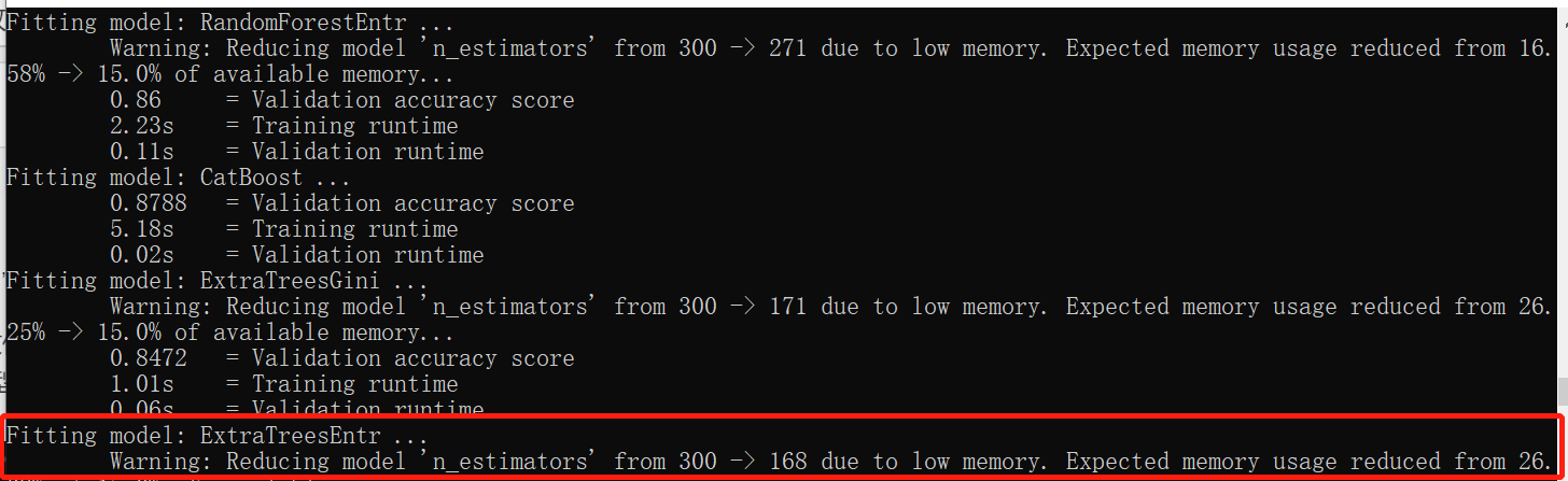
then... Hahaha, the notebook is too garbage. You can automatically adjust the parameters according to the memory

Load test set and verify

# load test set 
test_data = TabularDataset('https://autogluon.s3.amazonaws.com/datasets/Inc/test.csv')
y_test = test_data[label]  # values to predict
test_data_nolab = test_data.drop(columns=[label])  # delete label column to prove we're not cheating
test_data_nolab.head()
predictor = TabularPredictor.load(save_path)  # unnecessary, just demonstrates how to load previously-trained predictor from file

# model evalute 
y_pred = predictor.predict(test_data_nolab)
print("Predictions:  \n", y_pred)
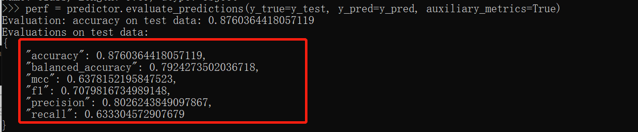
perf = predictor.evaluate_predictions(y_true=y_test, y_pred=y_pred, auxiliary_metrics=True)

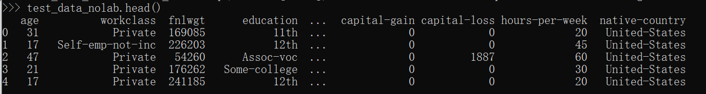
Let's show the data overview of the test set
Then there are the results. They are all basic model evaluation indicators. What I didn't expect is that the results of the same data and the same code training will be a little better than those on the official website. It may be due to different operating environments, but the difference is small, which is 4 percentage points worse

Demonstrate the effectiveness of all pre training models in the test set

predictor.leaderboard(test_data, silent=True)

From the classification accuracy, predictor Predict (test_data_nolab) uses weighensemble at this time_ L2 model
So far, the training of the first simple model has been completed, but I want to see the specific parameters of this model. This needs to be explored later, and I will release the follow-up tutorials. The first is the tutorial. If there are unreasonable places, please point out.

Show the accuracy of a particular classifier

predictor.predict(test_data, model='LightGBM')

Additional parts

Output prediction probability

pred_probs = predictor.predict_proba(test_data_nolab)
pred_probs.head(5)

What happens during fitting

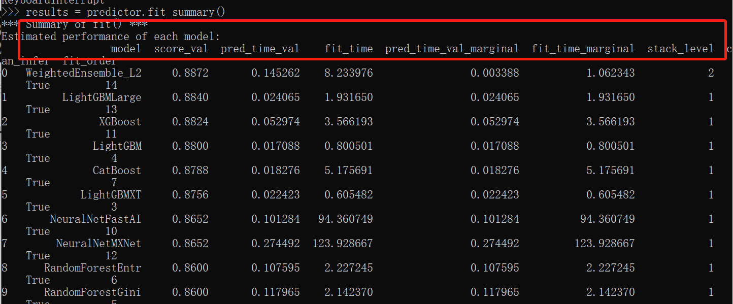
results = predictor.fit_summary()

Higher output accuracy

• time_limit: the longest waiting time for model training, which is usually not set
• eval_metric: evaluation index, AUC or accuracy, etc
• presets: defaults to 'medium'_ quality_ faster_ 'train 'loses accuracy, but it is fast. If it is set to "best_quality", bagging and stacking will be done to improve performance

time_limit = 60  # for quick demonstration only, you should set this to longest time you are willing to wait (in seconds)
metric = 'roc_auc'  # specify your evaluation metric here
predictor = TabularPredictor(label, eval_metric=metric).fit(train_data, time_limit=time_limit, presets='best_quality')
predictor.leaderboard(test_data, silent=True)