GOAL: to train a model on a variety of learning tasks, such that it can solve new learning tasks using only a small number of training samples.

Introduction: starting from face recognition, if a company has 50 people, it needs to make a face recognition system. According to the traditional deep learning idea, the recognition results should be divided into 51 categories (50 company members + 1 non company members). In order to train such a system, our data set needs to collect a large number of photos taken from various angles by these 50 company members and some non company members to train the neural network. But this is clearly not the case. When doing face recognition, you often only need company members to provide 1-2 photos. How? This is the method of today's feed shot learning. The goal of feed shot learning is to complete the classification through the input of small samples. In the term of feed shot learning, the data set of 50 people provided by the company is called Support Set, the 51 categories are called 51 way, the 1-2 photos provided by the company are called 1-shot or 2-shot, and the image data set collected in real time for face recognition is called query set.

(1 shot，6 way Support Set)

Common network models:

• Siamese network (twin network, improved version)

The work of the network mainly includes the following three processes:

        1. Pre training: the purpose is to train through a huge training set to learn and obtain an Embedding function for similarity feature extraction, which compresses a picture to a low dimensional vector, and the pictures of the same category or with similar features have similar vector values.

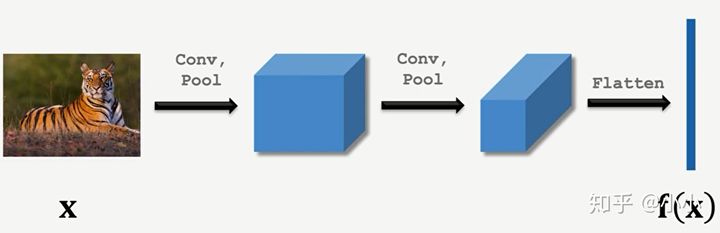
Embedding

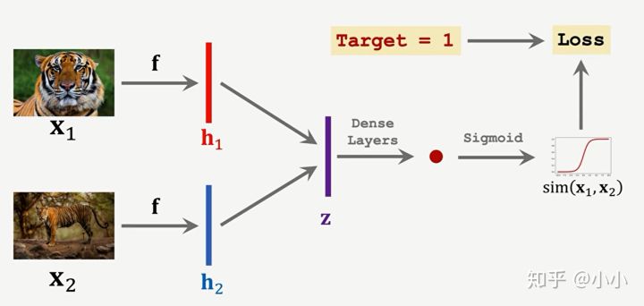
Pre training method 1: learning pair wise similarity score. The training sets are paired in pairs. After embedding, FC and Sigmoid respectively, if they are of the same kind, they are 1 and if they are not of the same kind, they are 0.

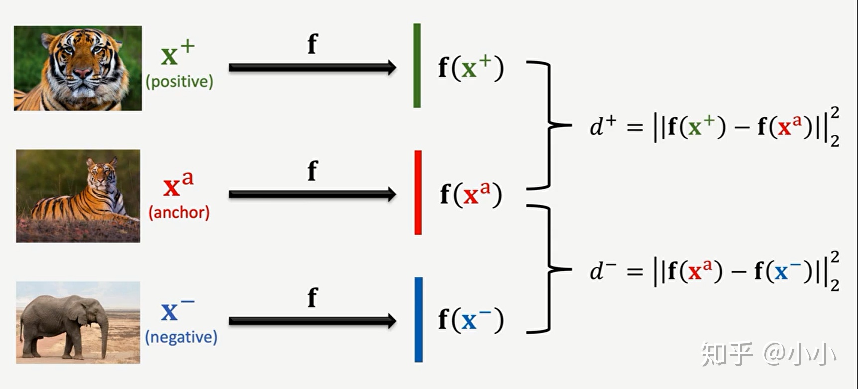
Pre training method 2: triple loss, randomly extract three images, one as anchor, one as positive image and the other as negative image. After embedding, calculate the similarity (distance, take two norm as an example) D1 and D2 between them and anchor image respectively, Then LOSS=max{0, d1-d2+ α }， Its meaning is that the similarity of images in the same category is greater than that in different categories.

        2. Fine tuning: the purpose is to fine tune the pre trained model according to the small Support Set in hand, so as to obtain better results.

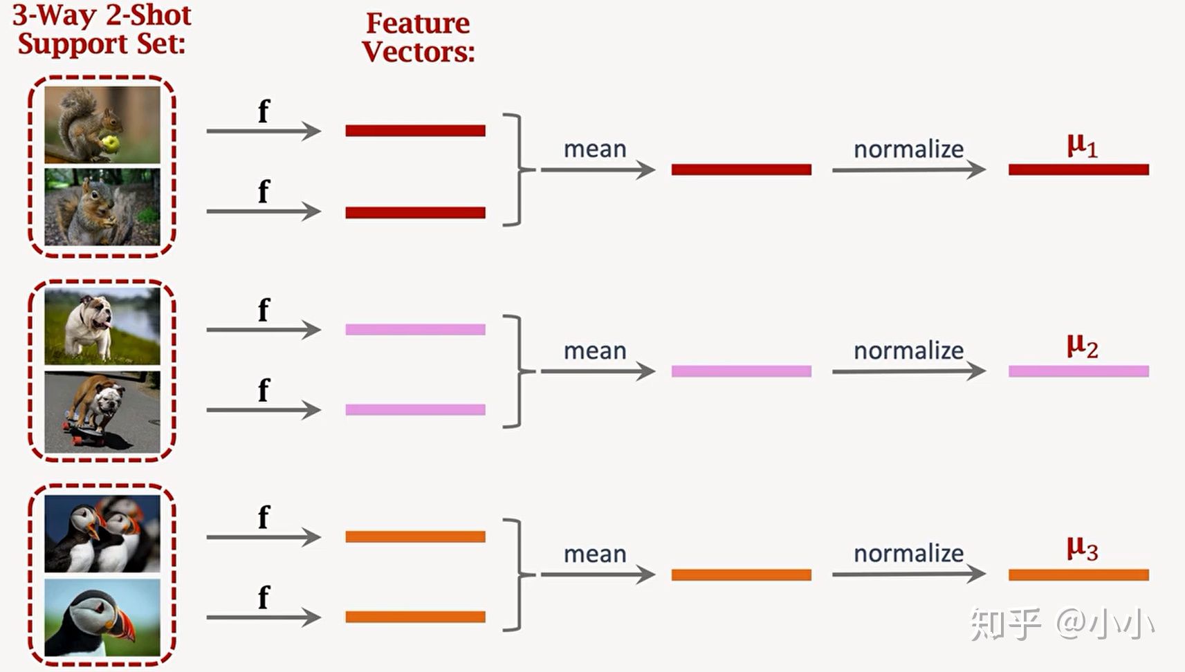
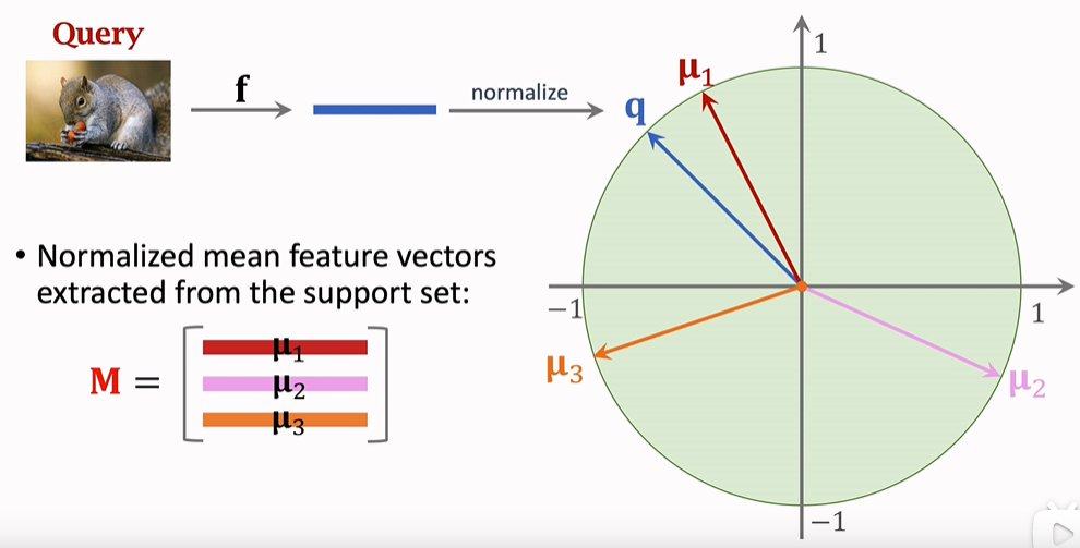
Firstly, embed the Support Set through the pre trained network, obtain the feature vector, and then normalize it to obtain the vector M=[ μ 1， μ 2， μ 3]

After obtaining the vector M, take the vector M as the initialization weight and the data (Xi, Yi) in the Support Set as the input to calculate the cosine distance to obtain the classification result. Compare the classification result with Yi to obtain the Loss function, so as to fine tune the classifier. Generally, the Loss function takes the cross entropy. In order to prevent over fitting, Regularization is usually performed, and the regularization function adopts Entropy Regulation.

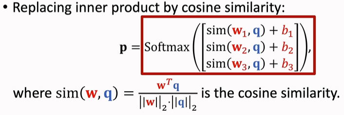
(in fine tuning, q in the picture should be changed to Xi)

 

        3. Test: use the model to test the random sample (query set) and observe its classification effect.

Reference: https://www.bilibili.com/video/BV1B44y1r75K/?spm_id_from=autoNext

• Matching Network

Paper: Matching Networks for One Shot Learning

In the paper, it is mentioned that the model mainly has two innovations: 1 In the model, attention (softmax) and memory (LSTM) are used to accelerate learning. 2 end to end learning of Test and train conditions must match for the same task

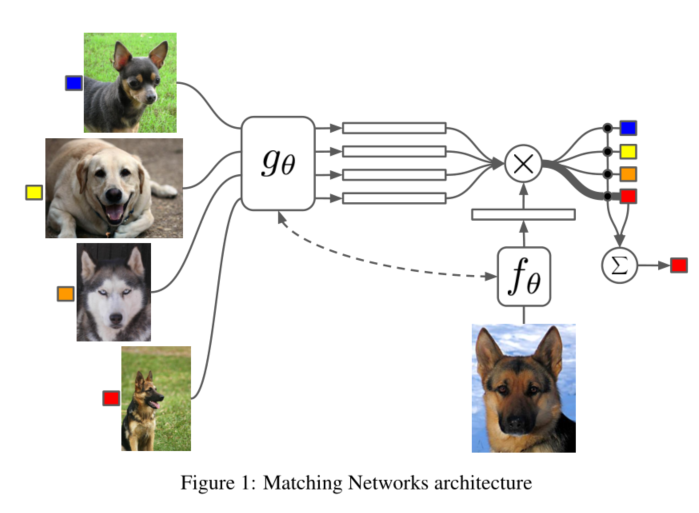
As shown in the figure above, g θ And f θ It is a feature extraction function, which compresses high-dimensional image data into feature vectors (embedding), usually using VGG or Inception network (later in the article, LSTM is also used to process CNN output, which is named "fully conditional embeddings, referred to as FCE), and {g θ And f θ Usually take the same network, but as mentioned in the paper, take different networks. The attention mechanism mentioned is mainly reflected in the second half of the network.

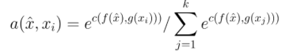
The above formula a(x,xi) represents attention, which is actually a softmax function, c(f(x),g(xi)) represents cosine similarity function, X cap represents the test input value of query set, and xi represents the sample of support set. The significance of this formula is to obtain the probability of which class the test sample belongs to.

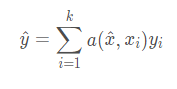
The above formula a(x,xi) is obtained from the above formula, yi is the category label corresponding to xi, one hot code, and y cap is the final predicted value.

For the FCE part, it mainly includes two parts: BidrectionalLSTM and {AttentionLSTM. The former is connected to support set and the latter is connected to query set. According to the author, this memory can improve learning efficiency. Its network structure is shown in the following code:

class MatchingNetwork(nn.Module):
    def __init__(self, n: int, k: int, q: int, fce: bool, num_input_channels: int,
                 lstm_layers: int, lstm_input_size: int, unrolling_steps: int, device: torch.device):
        """Creates a Matching Network as described in Vinyals et al.

        # Arguments:
            n: Number of examples per class in the support set
            k: Number of classes in the few shot classification task
            q: Number of examples per class in the query set
            fce: Whether or not to us fully conditional embeddings
            num_input_channels: Number of color channels the model expects input data to contain. Omniglot = 1,
                miniImageNet = 3
            lstm_layers: Number of LSTM layers in the bidrectional LSTM g that embeds the support set (fce = True)
            lstm_input_size: Input size for the bidirectional and Attention LSTM. This is determined by the embedding
                dimension of the few shot encoder which is in turn determined by the size of the input data. Hence we
                have Omniglot -> 64, miniImageNet -> 1600.
            unrolling_steps: Number of unrolling steps to run the Attention LSTM
            device: Device on which to run computation
        """
        super(MatchingNetwork, self).__init__()
        self.n = n
        self.k = k
        self.q = q
        self.fce = fce
        self.num_input_channels = num_input_channels
        self.encoder = get_few_shot_encoder(self.num_input_channels)
        if self.fce:
            self.g = BidrectionalLSTM(lstm_input_size, lstm_layers).to(device, dtype=torch.double)
            self.f = AttentionLSTM(lstm_input_size, unrolling_steps=unrolling_steps).to(device, dtype=torch.double)

    def forward(self, inputs):
        pass


class BidrectionalLSTM(nn.Module):
    def __init__(self, size: int, layers: int):
        """Bidirectional LSTM used to generate fully conditional embeddings (FCE) of the support set as described
        in the Matching Networks paper.

        # Arguments
            size: Size of input and hidden layers. These are constrained to be the same in order to implement the skip
                connection described in Appendix A.2
            layers: Number of LSTM layers
        """
        super(BidrectionalLSTM, self).__init__()
        self.num_layers = layers
        self.batch_size = 1
        # Force input size and hidden size to be the same in order to implement
        # the skip connection as described in Appendix A.1 and A.2 of Matching Networks
        self.lstm = nn.LSTM(input_size=size,
                            num_layers=layers,
                            hidden_size=size,
                            bidirectional=True)

    def forward(self, inputs):
        # Give None as initial state and Pytorch LSTM creates initial hidden states
        output, (hn, cn) = self.lstm(inputs, None)

        forward_output = output[:, :, :self.lstm.hidden_size]
        backward_output = output[:, :, self.lstm.hidden_size:]

        # g(x_i, S) = h_forward_i + h_backward_i + g'(x_i) as written in Appendix A.2
        # AKA A skip connection between inputs and outputs is used
        output = forward_output + backward_output + inputs
        return output, hn, cn


class AttentionLSTM(nn.Module):
    def __init__(self, size: int, unrolling_steps: int):
        """Attentional LSTM used to generate fully conditional embeddings (FCE) of the query set as described
        in the Matching Networks paper.

        # Arguments
            size: Size of input and hidden layers. These are constrained to be the same in order to implement the skip
                connection described in Appendix A.2
            unrolling_steps: Number of steps of attention over the support set to compute. Analogous to number of
                layers in a regular LSTM
        """
        super(AttentionLSTM, self).__init__()
        self.unrolling_steps = unrolling_steps
        self.lstm_cell = nn.LSTMCell(input_size=size,
                                     hidden_size=size)

    def forward(self, support, queries):
        # Get embedding dimension, d
        if support.shape[-1] != queries.shape[-1]:
            raise(ValueError("Support and query set have different embedding dimension!"))

        batch_size = queries.shape[0]
        embedding_dim = queries.shape[1]

        h_hat = torch.zeros_like(queries).cuda().double()
        c = torch.zeros(batch_size, embedding_dim).cuda().double()

        for k in range(self.unrolling_steps):
            # Calculate hidden state cf. equation (4) of appendix A.2
            h = h_hat + queries

            # Calculate softmax attentions between hidden states and support set embeddings
            # cf. equation (6) of appendix A.2
            attentions = torch.mm(h, support.t())
            attentions = attentions.softmax(dim=1)

            # Calculate readouts from support set embeddings cf. equation (5)
            readout = torch.mm(attentions, support)

            # Run LSTM cell cf. equation (3)
            # h_hat, c = self.lstm_cell(queries, (torch.cat([h, readout], dim=1), c))
            h_hat, c = self.lstm_cell(queries, (h + readout, c))

        h = h_hat + queries

        return h

• Prototype networks

paper: Prototypical Networks for Few-shot Learning

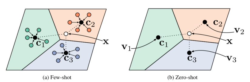
The advantage is that it is very simple, and according to the article, it has similar accuracy to the Matching Network. Its basic idea is consistent with kNN (nearest neighbor algorithm), which mainly includes the following three processes:

1) embedding, compressing the image (feed shot, left) or the described meta information (zero shot, meta learning, right) into a low-dimensional feature vector;

 

def get_few_shot_encoder(num_input_channels=1) -> nn.Module:
    """Creates a few shot encoder as used in Matching and Prototypical Networks

    # Arguments:
        num_input_channels: Number of color channels the model expects input data to contain. Omniglot = 1,
            miniImageNet = 3
    """
    return nn.Sequential(
        conv_block(num_input_channels, 64),
        conv_block(64, 64),
        conv_block(64, 64),
        conv_block(64, 64),
        Flatten(),
    )

def conv_block(in_channels: int, out_channels: int) -> nn.Module:
    """Returns a Module that performs 3x3 convolution, ReLu activation, 2x2 max pooling.

    # Arguments
        in_channels:
        out_channels:
    """
    return nn.Sequential(
        nn.Conv2d(in_channels, out_channels, 3, padding=1),
        nn.BatchNorm2d(out_channels),
        nn.ReLU(),
        nn.MaxPool2d(kernel_size=2, stride=2)
    )

2) for each category (way/class) of the Support Set, calculating the class prototype of its eigenvector is actually a process of solving the mean value:

def compute_prototypes(support: torch.Tensor, k: int, n: int) -> torch.Tensor:
    """Compute class prototypes from support samples.

    # Arguments
        support: torch.Tensor. Tensor of shape (n * k, d) where d is the embedding
            dimension.
        k: int. "k-way" i.e. number of classes in the classification task
        n: int. "n-shot" of the classification task

    # Returns
        class_prototypes: Prototypes aka mean embeddings for each class
    """
    # Reshape so the first dimension indexes by class then take the mean
    # along that dimension to generate the "prototypes" for each class
    class_prototypes = support.reshape(k, n, -1).mean(dim=1)
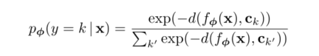
    return class_prototypes

3) for data X of Query Set, calculating the probability of belonging to each category is actually a calculation of Softmax, but it is worth mentioning that Bregman divergence (i.e. Euclidean distance) should be used to calculate the similarity in the paper

def pairwise_distances(x: torch.Tensor,
                       y: torch.Tensor,
                       matching_fn: str) -> torch.Tensor:
    """Efficiently calculate pairwise distances (or other similarity scores) between
    two sets of samples.

    # Arguments
        x: Query samples. A tensor of shape (n_x, d) where d is the embedding dimension
        y: Class prototypes. A tensor of shape (n_y, d) where d is the embedding dimension
        matching_fn: Distance metric/similarity score to compute between samples
    """
    n_x = x.shape[0]
    n_y = y.shape[0]

    if matching_fn == 'l2':
        distances = (
                x.unsqueeze(1).expand(n_x, n_y, -1) -
                y.unsqueeze(0).expand(n_x, n_y, -1)
        ).pow(2).sum(dim=2)
        return distances
    elif matching_fn == 'cosine':
        normalised_x = x / (x.pow(2).sum(dim=1, keepdim=True).sqrt() + EPSILON)
        normalised_y = y / (y.pow(2).sum(dim=1, keepdim=True).sqrt() + EPSILON)

        expanded_x = normalised_x.unsqueeze(1).expand(n_x, n_y, -1)
        expanded_y = normalised_y.unsqueeze(0).expand(n_x, n_y, -1)

        cosine_similarities = (expanded_x * expanded_y).sum(dim=2)
        return 1 - cosine_similarities
    elif matching_fn == 'dot':
        expanded_x = x.unsqueeze(1).expand(n_x, n_y, -1)
        expanded_y = y.unsqueeze(0).expand(n_x, n_y, -1)

        return -(expanded_x * expanded_y).sum(dim=2)
    else:
        raise(ValueError('Unsupported similarity function'))

• MAML (model agnostic meta learning)

paper: Model-Agnostic Meta-Learning for Fast Adaptation of Deep Networks

With regard to model agnostic, the author said: it is applicable to any model using gradient descent, including classification, regression and reinforcement learning.

Core idea: train the initial parameters of the model, so that these parameters can get good results after one or more gradient updates in the small data of the new task.

Do you think the above two descriptions are very mysterious but a little cowhide? Both are literal translations of the author's original text. The first half of this paper is frantically repeating the above two views with various expressions, playing tricks and playing tricks. In fact, the description of the core content is so little. It mainly includes the following three steps:

First, a large data set (task) T is divided into many small data sets (task) Ti (meta batch), and the data set (task) Ti is divided into two parts, K samples and N-K samples respectively;

    for meta_batch in x:
        # By construction x is a 5D tensor of shape: (meta_batch_size, n*k + q*k, channels, width, height)
        # Hence when we iterate over the first  dimension we are iterating through the meta batches
        x_task_train = meta_batch[:n_shot * k_way]
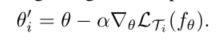
        x_task_val = meta_batch[n_shot * k_way:]

Second, a model weight parameter is generated by random initialization θ， For each small data set (task) Ti, K þ samples in the data set are extracted for training, and a new weight parameter of the model corresponding to the small data set is updated by gradient descent method θ i:

        # Train the model for `inner_train_steps` iterations
        for inner_batch in range(inner_train_steps):
            # Perform update of model weights
            y = create_nshot_task_label(k_way, n_shot).to(device)
            logits = model.functional_forward(x_task_train, fast_weights)
            loss = loss_fn(logits, y)
            gradients = torch.autograd.grad(loss, fast_weights.values(), create_graph=create_graph)

            # Update weights manually
            fast_weights = OrderedDict(
                (name, param - inner_lr * grad)
                for ((name, param), grad) in zip(fast_weights.items(), gradients)  # zip package into meta group
            )

Third, after training each small data set (task) Ti ， a new weight parameter of the model will be obtained θ i. Take the remaining N-K data samples of the data set based on the new weight parameters θ i. Calculate the ， Loss ， and ， gradients corresponding to each small data set:

        # Do a pass of the model on the validation data from the current task
        # Test the updated parameters with the test set and save the task_predictions and tasks_ Losses and tasks_ gradients
        y = create_nshot_task_label(k_way, q_queries).to(device)
        logits = model.functional_forward(x_task_val, fast_weights)
        loss = loss_fn(logits, y)
        loss.backward(retain_graph=True)

        # Get post-update accuracies
        y_pred = logits.softmax(dim=1)
        task_predictions.append(y_pred)

        # Accumulate losses and gradients
        task_losses.append(loss)
        gradients = torch.autograd.grad(loss, fast_weights.values(), create_graph=create_graph)
        named_grads = {name: g for ((name, _), g) in zip(fast_weights.items(), gradients)}
        task_gradients.append(named_grads)

Then, sum up these different small data ＾ Ti ＾ gradient ＾ (this code can't understand, woo woo)

sum_task_gradients = {k: torch.stack([grad[k] for grad in task_gradients]).mean(dim=0)
                                  for k in task_gradients[0].keys()}
hooks = []
for name, param in model.named_parameters():
    hooks.append(
        param.register_hook(replace_grad(sum_task_gradients, name))
    )

Finally, update the weight based on the summed gradient parameters. The parameters in the model() function are defined as:

def __init__(self, num_input_channels: int, k_way: int, final_layer_size: int = 64)

And when did you pass in the gradient parameters of the previous summation???)

            model.train()
            optimiser.zero_grad()
            # Dummy pass in order to create `loss` variable
            # Replace dummy gradients with mean task gradients using hooks
            logits = model(torch.zeros((k_way, ) + data_shape).to(device, dtype=torch.double))
            loss = loss_fn(logits, create_nshot_task_label(k_way, 1).to(device))
            loss.backward()
            optimiser.step()

            for h in hooks:
                h.remove()

Code source: https://github.com/oscarknagg/few-shot

---------------------------

---------------------------

---------Bald head jpg--------

----------------------------

----------------------------

• My understanding:
• Why is MAML suitable for small data? Because if we train directly, the data set is very small, the training will be completed in a short time, and the model is not very good. Therefore, the author adopts a mechanism of random combination sampling of categories to make multiple use of the data;
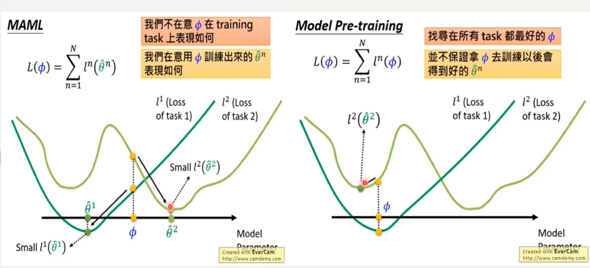
• Why does meta update add and then derive the Loss function based on Task batch instead of direct gradient descent? Because the ideal result of directly using gradient descent is to make the solution converge to the local optimal solution, but MAML does not want this. It wants better adaptability, that is, when a new task comes in, it will converge to the optimal solution of the new task through iteration as much as possible, Therefore, training should reach an "intermediate position", so sum and derivative are used (the operations of derivation and sum can be exchanged).

• What do you mean by first order and second order in the paper? Why does meta update use the original parameters θ Not the optimized parameters θ i derivative?

The derivation process comes from: https://www.bilibili.com/video/BV11E411G7V9

 

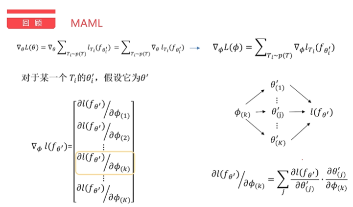
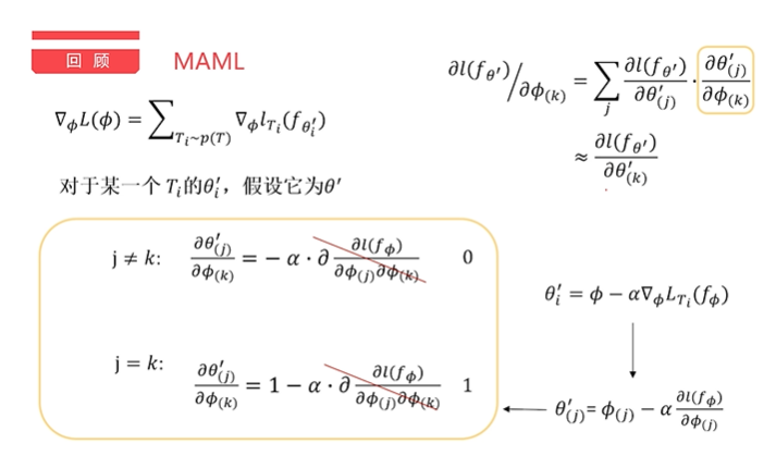
The results show that if the influence of the second order is ignored, the final result is equivalent to the optimized result of the Loss function θ So what is the impact or advantage of second order? Actually, i don't know.