-
Bayesian theory
-
Continuous and discrete feature processing
-
Naive Bayes classifier
-
Semi naive Bayesian classifier
Bayesian theory
In our study of probability theory, Bayesian theory is basically implied everywhere. Bayesian theory is simply a method of probability transformation, which transforms a difficult correlation probability into several easier probability products.
Now let's consider a classification task. There are N categories. We will classify them as
c
j
c_j
The sample of cj ^ is incorrectly divided into
c
i
c_i
The loss of ci is defined as
λ
i
j
λ_{ij}
λ ij, a posteriori probability
P
(
c
i
∣
x
)
P(c_i|x)
P(ci ∣ x) indicates that sample x is divided into
c
i
c_i
The probability of ci. Through the above formula, we can calculate an expected loss, that is, an estimate of the overall expected loss. It is also called conditional risk.
R
(
c
i
∣
x
)
=
∑
j
=
1
N
λ
i
j
P
(
c
j
∣
x
)
R(c_i|x)=\sum_{j=1}^Nλ_{ij}P(c_j|x)
R(ci∣x)=∑j=1NλijP(cj∣x)
From the formula, it can be understood that the expected loss = misjudgment loss of unit category * discrimination probability of a single sample
As can be seen from the above, now R is our objective function, representing the theoretical loss of the whole discriminant theory, and our goal is to minimize the loss function, that is, to find the most appropriate one for each sample; The category tag minimizes R. take
h
(
x
)
h(x)
h(x) is recorded as Bayesian optimal classifier
h
(
x
)
=
a
r
g
m
i
n
R
(
c
∣
x
)
h(x)=argminR(c|x)
h(x)=argminR(c∣x)
. Now let's measure it by 0-1 loss
λ
i
j
λ_{ij}
λij
λ
i
j
=
{
1
Category prediction error
0
Category prediction is correct
λ_ {ij} = \ left \ {\ begin {aligned} 1 & & \ text {category prediction error} \ \ 0 & & \ text {category prediction correct} \ end{aligned} \right
λ ij = {10} category prediction error category prediction is correct
Then R is:
R
(
c
i
∣
x
)
=
∑
j
=
1
N
P
(
c
j
∣
x
)
−
sentence
yes
General
rate
R(c_i|x)=\sum_{j=1}^NP(c_j|x) - judgment probability
R(ci ∣ x) = ∑ j=1N ∣ P(cj ∣ x) − judgment probability
=
∑
j
=
1
N
P
(
c
j
∣
x
)
−
P
(
c
∣
x
)
=\sum_{j=1}^NP(c_j|x)-P(c|x)
=∑j=1NP(cj∣x)−P(c∣x)
=
1
−
P
(
c
∣
x
)
=1-P(c|x)
=1−P(c∣x)
From the above h(x), it can be seen that minimizing h(x) is equal to minimizing R, so
h
(
x
)
=
a
r
g
m
i
n
R
(
c
∣
x
)
=
a
r
g
m
i
n
(
1
−
P
(
c
∣
x
)
)
=
a
r
g
m
a
x
P
(
c
∣
x
)
h(x)=argminR(c|x)=argmin(1-P(c|x))=argmaxP(c|x)
h(x)=argminR(c∣x)=argmin(1−P(c∣x))=argmaxP(c∣x)
Therefore, finding the best Bayesian classifier is the required posterior probability
P
(
c
∣
x
)
P(c|x)
P(c∣x)
Bayes theorem:
P
(
c
∣
x
)
=
P
(
c
)
P
(
x
∣
c
)
P
(
x
)
)
P(c|x)=\frac{P(c)P(x|c)}{P(x))}
P(c∣x)=P(x))P(c)P(x∣c)
For a given total sample D, a single sample P(x) is the same for all class markers, so the core concern is molecules. For
P
(
c
)
P(c)
P(c) we can use the large number theorem to estimate according to the frequency of samples. But conditional probability
P
(
x
∣
c
)
P(x|c)
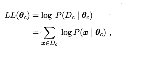
P(x ∣ c) involves the joint probability of all attributes of the sample, which is not easy to obtain directly. Usually, we assume that it obeys a certain probability distribution, and estimate the parameters of the probability distribution based on the training samples. In general, we use log maximum likelihood estimation to solve it.
Premise: assuming that it obeys a certain distribution (we assume that its probability density function is known), it is independent and identically distributed
hypothesis
P
(
x
∣
c
)
P(x|c)
P(x ∣ c) has a definite form and is parameterized
θ
c
θ_c
θ c) uniquely determined,
D
c
D_c
Dc ﹤ represents the sum of samples with category c in sample D

We take logarithms on both sides respectively to prevent underflow caused by excessive continuous power
Finally, we can use the assumed probability density distribution to replace the two pairs θ The final maximum likelihood estimate is calculated by derivation θ (maximum likelihood function solution method in high numbers). If we assume that this is a normal distribution, then θ It refers to in the normal distribution
u
c
,
δ
c
2
u_c,\delta_c^2
uc, δ c2, calculated:

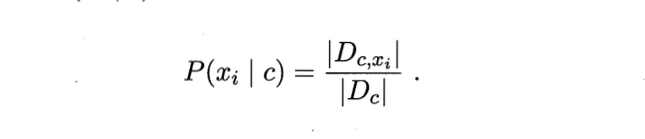
Continuous value and discrete value processing
For discrete values, our processing method is very simple. We only need to take the value of the ith attribute as
x
i
x_i
xi. The set of samples can be compared with the number of samples
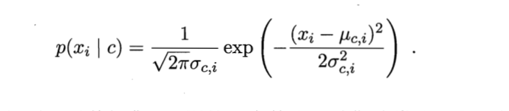
For continuous values, this cannot be done. For continuous values, we generally have the following two processing methods:
1: Barrel separation method
We divide the data into different m segments and calculate a probability for each segment, but this will be greatly affected by the size of m value
2: Hypothetical probability distribution method:
We can assume that it obeys a certain probability distribution, and then use its probability density distribution function to calculate it. In this way, the probability problem of finding continuous values is transformed into the area problem under the influence of values. If it obeys normal distribution, we can calculate it as follows:
Naive Bayes classifier
Premise: independent and identically distributed
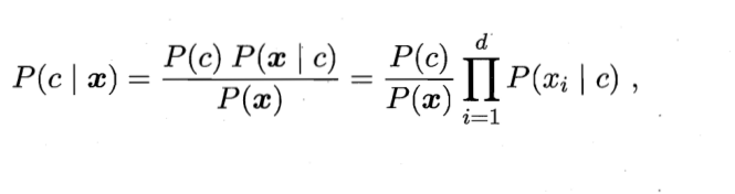
In a word, there is no connection between features (although it is not in line with the actual situation), which can be transformed into the form of probability multiplication of single conditional features. However, this will also bring a problem. Once a feature has not appeared in a class, the result of its multiplication will be 0. This will cause that no matter how other attributes of the sample change, it will eventually be 0, which is obviously inconsistent with the fact. "Not observed" and "probability of occurrence is 0" are two very different situations. In order to smooth the probability, we generally adopt Laplace correction:
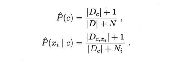
Parameter introduction:
Dc: sample D Category in is c Sample set for
N:D Number of possible categories in
Ni:Number i Possible values of attributes
Dc,xi: Dc pass the civil examinations i Attribute values are xi Sample set for
+1: The prevention molecule is 0
sklearn provides us with four Bayesian classification functions (Bernoulli, supplementary Bayes, Gauss and polynomial) and a Bayesian regression function (linear. Model. Bayesian ridge)
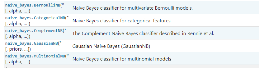
The following is a text classification case to show the effect of Bayesian classifier under Gaussian distribution
from sklearn.model_selection import train_test_split
from sklearn.naive_bayes import GaussianNB
from sklearn.feature_extraction.text import CountVectorizer,TfidfVectorizer
import pandas as pd
import jieba
import numpy as np
# get data
dataset = pd.read_table(r'./dataset.txt',names=['category','theme','URL','content'],encoding='utf-8')
dataset.head(-1)
# Get article content
content = dataset.content.values.tolist()
# content
# Content participle
segment_words = list()
for line in content:
    segment = jieba.lcut(line)
    if len(segment)>1 and segment!="\r\n":
        segment_words.append(segment)
segment_words[1000]

contents = pd.DataFrame({"content":segment_words})
contents = contents.content.values.tolist()
# Remove the contents of the stoplist
stopwords = pd.read_table(r'./stopwords.txt',quoting=3,names=["stopwords"],encoding='utf-8')
stopwords = stopwords.stopwords.values.tolist()

new_content = list()
for line in contents:
    line_content = list()
    for word in line:
        if word in stopwords:
            continue
        line_content.append(word)
    new_content.append(line_content)
df_train=pd.DataFrame({'content':new_content,'label':dataset['category']})
df_train.head()
# Class tag discretization
label_mapping = {"automobile": 1, "Finance and Economics": 2, "science and technology": 3, "healthy": 4, "Sports":5, "education": 6,"Culture": 7,"military": 8,"entertainment": 9,"fashion": 0}
df_train.label = df_train['label'].map(label_mapping)
# Data segmentation
x_train,x_test,y_train,y_test = train_test_split(df_train.content.values,df_train.label.values,test_size=0.2,random_state=100)

train_content = list()
# The training set is transformed into list of str form u, which is convenient for subsequent feature coding
for line_index in range(len(x_train)):
	train_content.append(' '.join(x_train[line_index]))

# Feature coding to form a sparse matrix
transfer = CountVectorizer(analyzer="word",max_features=4000)
x_train = transfer.fit_transform(train_content)

# Training model
estimator = GaussianNB()
estimator.fit(x_train.toarray(),y_train)
# Test set data coding
train= list()
for index in range(len(x_test)):
    train.append(" ".join(x_test[index]))
#transfer1 = TfidfVectorizer()
transfer1 = CountVectorizer(analyzer="word",max_features=4000)
x_test = transfer1.fit_transform(train)
estimator.score(x_test.toarray(),y_test)
Semi naive Bayesian classifier
In naive Bayesian classifier, we assume that the premise is independent and identically distributed, but in reality, this condition is difficult to hold, and there will be more or less connections between features. In order to improve this defect, semi naive Bayesian classifiers mostly adopt the strategy of independent dependence estimation, that is, each attribute designed now depends on at most one other attribute:

p
a
i
pa_i
pai is
x
i
x_i
xi , the dependent attribute is called parent attribute (super parent). There are many methods of semi Bayesian classifier. Its essential idea is how to measure the correlation between features, and then a new method to calculate conditional probability is proposed.
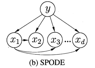
Above SPODE The single super parent method assumes that the other features are independent of each other, and all features are related to the unique features.
Nowadays, there is a more powerful semi Bayesian classifier based on ensemble learning mechanism AODE,Is in SPODE Change a single superparent into all superparents on the basis of,
That is to say, one of the features is now separately SPODE Method, each feature acts as a superparent once. The formula is as follows:
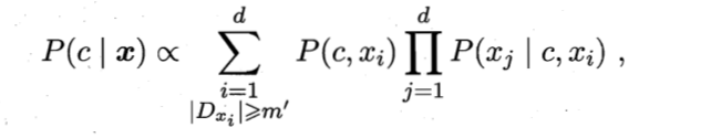
The essence is to aggregate multiple SPODE models based on the integration mechanism, and finally propose the following probability calculation method:
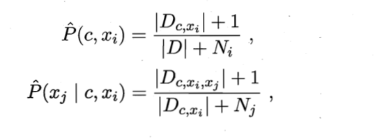
D: Total sample set
Ni:Number i Possible values of attributes
Dc,xi: Dc pass the civil examinations i Attribute values are xi Sample set for
Dc,xi,xj: D Category in is c And the first i,j Attribute values are xi,xj Sample set for
+1: The prevention molecule is 0