123. Best Time to Buy and Sell Stock III
You are given an array prices where prices[i] is the price of a given stock on the ith day.
Find the maximum profit you can achieve. You may complete at most two transactions.
Note: You may not engage in multiple transactions simultaneously (i.e., you must sell the stock before you buy again).
Example 1:
Input: prices = [3,3,5,0,0,3,1,4]
Output: 6
Explanation: Buy on day 4 (price = 0) and sell on day 6 (price = 3), profit = 3-0 = 3.
Then buy on day 7 (price = 1) and sell on day 8 (price = 4), profit = 4-1 = 3.
Example 2:
Input: prices = [1,2,3,4,5]
Output: 4
Explanation: Buy on day 1 (price = 1) and sell on day 5 (price = 5), profit = 5-1 = 4.
Note that you cannot buy on day 1, buy on day 2 and sell them later, as you are engaging multiple transactions at the same time. You must sell before buying again.
Example 3:
Input: prices = [7,6,4,3,1]
Output: 0
Explanation: In this case, no transaction is done, i.e. max profit = 0.
Example 4:
Input: prices = [1]
Output: 0
Constraints:
- 1 <= prices.length <= 105
- 0 <= prices[i] <= 105
1. Logic analysis of buying low and selling high
At first, the part where we calculated minimumBuyPrice2 confused me. Then I tried to study mathematics myself and see what happened. I hope the following explanation will help people who are equally confused with me.
Therefore, in the following code, lowestBuyPrice1 and maxProfit1 are easy to understand. The only thing that may take time to understand is the calculation of minimum purchase price 2. minimumBuyPrice2 here is not actually the exact price at which we bought the stock in the second transaction. In fact, if we can open it, it contains two parts
"lowestBuyPrice2" = buyPrice2 - maxProfit1
                  = buyPrice2 - (highestSellPrice1 - lowestBuyPrice1).
So you will see that "lowestBuyPrice2" includes the purchase price of the second transaction and the profit from our first transaction. When we calculate
"maxProfit2" = sellPrice2 - lowestBuyPrice2
             = sellPrice2 - buyPrice2 + maxProfit1
             = profitOf2ndTrans + maxProfit1.
Therefore, at the end of the calculation, "maxProfit2" will contain the profits of the two transactions.
To avoid ambiguity in the names used for these variables, I use italics to separate variables ("lowestBuyPrice2", "maxProfit2"), and the meaning of these variables may be confusing.
The final solution is as follows:
public class Solution {
    public int maxProfit(int[] prices) {
        int maxProfit1 = 0;
        int maxProfit2 = 0;
        int lowestBuyPrice1 = Integer.MAX_VALUE;
        int lowestBuyPrice2 = Integer.MAX_VALUE;

        for(int p:prices){
            maxProfit2 = Math.max(maxProfit2, p-lowestBuyPrice2);
            lowestBuyPrice2 = Math.min(lowestBuyPrice2, p-maxProfit1);
            maxProfit1 = Math.max(maxProfit1, p-lowestBuyPrice1);
            lowestBuyPrice1 = Math.min(lowestBuyPrice1, p);
        }
        return maxProfit2;
    }
}
2. Expand to K transactions
The above two transactions are special cases and can be extended to the following general methods.
class Solution {
    public int maxProfit(int[] prices) {
        return maxProfit(2, prices);
    }

    public int maxProfit(int k, int[] prices) {
        int[] s = new int[k+1];
        int[] b = new int[k+1];
        for(int i=0; i<b.length; i++)
            b[i] = Integer.MIN_VALUE;
        for(int p : prices) {
            for(int i=k; i>=1; i--) {
                s[i] = Math.max(s[i], b[i]+p);
                b[i] = Math.max(b[i], s[i-1]-p);
            }
        }
        return s[k];
    }
}
3. Simple DP solution of state machine, O(n) time complexity, O(1) space complexity
This method can be used for all stock price based problems.
The idea is to design a state machine that correctly describes the problem statement.
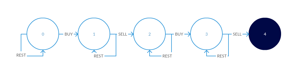
Intuition behind the state diagram:
We start with state 0, where we can rest (i.e. do nothing) or buy stocks at a given price.
- If we choose to rest, we keep our state 0
- If we buy, we spend some money (the stock price of the day) and then go to state 1
From state 1, we can choose to do nothing again, or we can sell our shares.
- If we choose to rest, we stay in shape 1
- If we sell, we make some money (the stock price of the day) and then go to state 2
This closed a deal for us. Remember, the only atmosphere 2 deal we can do.
From the state 2, we can choose to do nothing or buy more stocks.
- If we choose to rest, we keep in shape 2
- If we buy, we go to state 3
From state 3, we can choose to do nothing again, or we can sell our shares for the last time.
- If we choose to rest, we stay in shape 3
- If we sell, we have taken advantage of the transactions we allow and reached the final state 4
From state diagram to code
// Assume we are in state S
// If we buy, we are spending money but we can also choose to do nothing
// Doing nothing means going from S->S
// Buying means going from some state X->S, losing some money in the process
S = max(S, X-prices[i])

// Similarly, for selling a stock
S = max(S, X+prices[i])
code:
int maxProfit(vector<int>& prices) {
	if(prices.empty()) return 0;
	int s1=-prices[0],s2=INT_MIN,s3=INT_MIN,s4=INT_MIN;

	for(int i=1;i<prices.size();++i) {
		s1 = max(s1, -prices[i]);
		s2 = max(s2, s1+prices[i]);
		s3 = max(s3, s2-prices[i]);
		s4 = max(s4, s3+prices[i]);
	}
	return max(0,s4);
}
We can create four variables, one for each state, excluding the initial state, because it is always 0, initialization s1 is - prices[0], and the rest is INT_MIN because they will be overwritten later.
To achieve s1, we either stay where we are or s1 buy stocks for the first time.
In order to reach s2, we either stay inside, s2 or we sell, s1 and then to s2
Similarly, s3 and s4.
Finally, we return s4 or, more precisely, max(0,s4) because we initialize s4 to INT_MIN.
This idea applies to all problems of stocks. As long as our state diagram is correct, we can code it like this.
Side note: technically speaking, this is a dynamic programming method. We should actually do this. s2[i] = max(s2[i-1], s1[i-1]+prices[i]) but we can rest assured that the coverage value s1 will always be better than the previous one, so we don't need temporary variables.
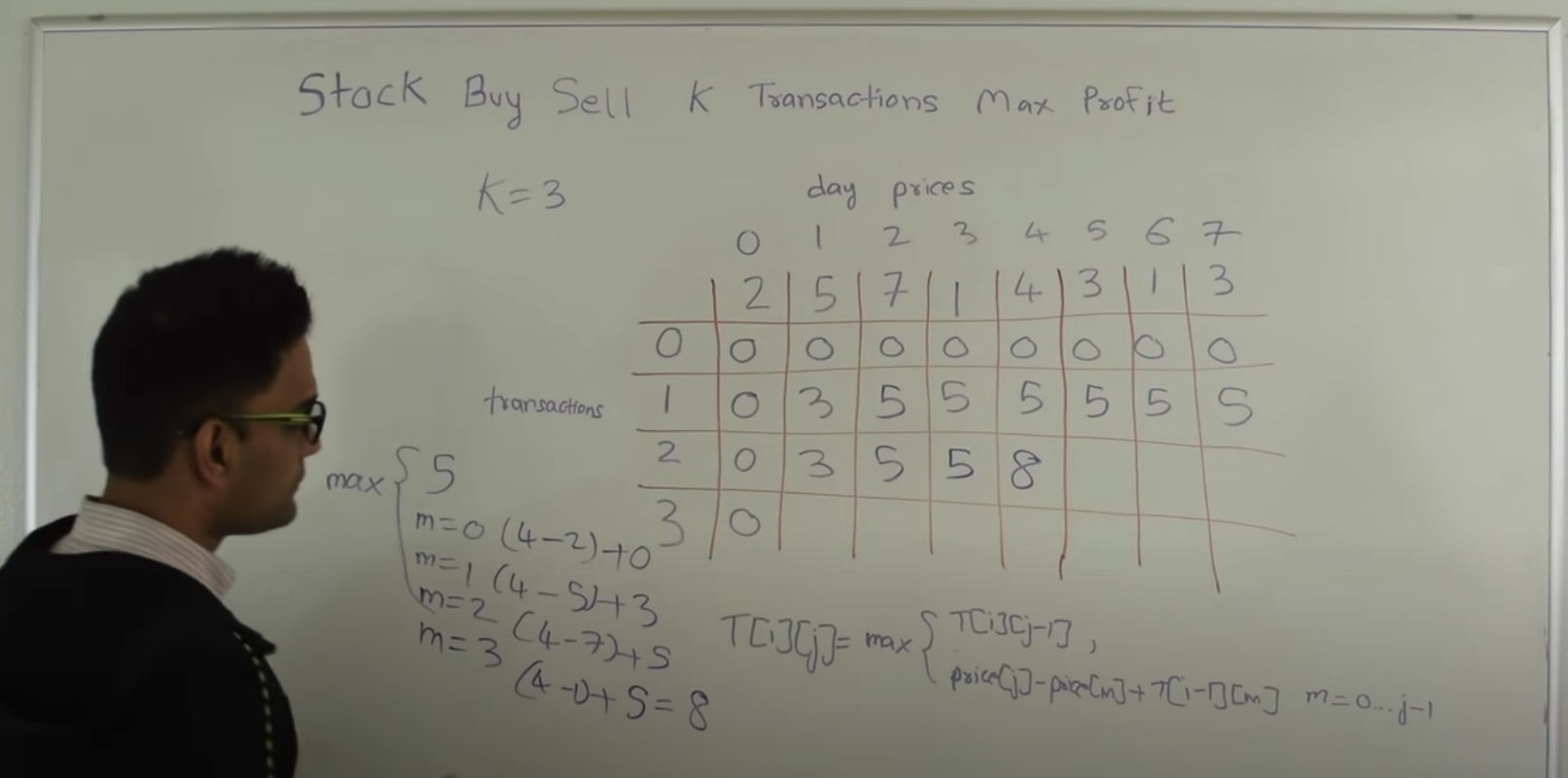
4. Dynamic programming – deduction from 1 transaction to 3 transactions at most
https://www.youtube.com/watch?v=oDhu5uGq_ic&ab_channel=CodingTech
It is not difficult to get DP recursive formula:
dp[k, i] = max(dp[k, i-1], prices[i] - prices[j] + dp[k-1, j-1]), j=[0..i-1]
For k transactions, on day i,
If we do not trade, the profit is the same as the previous day dp[k, i-1];
If we buy stocks on day J, where j=[0..i-1], and then sell stocks on day I, the profit is prices [i] - prices [J] + DP [k-1, J-1].
In fact, j can also be I. When j is I, another commodity prices[i] -prices[j] + dp[k-1, j] = dp[k-1, i] looks like we just lost a trading opportunity.
I see others use the formula dp[k, i] = max(dp[k, i-1],prices[i] -prices[j] + dp[k-1, j]), and the last one is dp[k-1, j] instead of dp[k-1, j-1]. This is not in a direct sense. If the stock is bought on day j, the total profit of the previous transaction should be completed on day (j-1). However, the result based on this formula is also correct, because if the stock is sold on day j and then bought again, the result is the same if we don't trade on that day.
Therefore, the direct implementation is:
4.1 the time complexity is O(kn^2) and the space complexity is O(kn).
class Solution {
    public int maxProfit(int[] prices) {
        int n=prices.length;
        if(n==0) return 0;
        int[][] dp=new int[3][n];
        for (int k=1;k<=2;k++){
            for (int i=1;i<n;i++){
                int min=prices[0];
                for (int j=1;j<=i;j++){
                    min=Math.min(min, prices[j]-dp[k-1][j-1]);
                }
                dp[k][i] = Math.max(dp[k][i-1], prices[i] - min);
            }
        }
        return dp[2][n-1];
    }
}
4.2 in the above code, min is calculated repeatedly. It can be easily improved to:
The time complexity is O(kn) and the space complexity is O(kn).
class Solution {
    public int maxProfit(int[] prices) {
        int n=prices.length;
        if(n==0) return 0;
        int[][] dp=new int[3][n];
        for (int k=1;k<=2;k++){
            int min=prices[0];
            for (int i=1;i<n;i++){
                min=Math.min(min, prices[i]-dp[k-1][i-1]);
                dp[k][i] = Math.max(dp[k][i-1], prices[i] - min);
            }
        }
        return dp[2][n-1];
    }
}
4.3 we need to save min for each transaction, so there are k "Min".
We can find that the second dimension (variable I) only depends on the previous dimension (i-1), so we can compress this dimension. (we can also select the first dimension (Variable k) because it also depends only on the previous dimension k-1, but we can't compress the two dimensions at the same time.)
Therefore, the time complexity is O(kn), and the space complexity becomes O(k).
class Solution {
    public int maxProfit(int[] prices) {
        int n=prices.length;
        if(n==0) return 0;
        int[][] dp=new int[3][n];
        int[] min=new int[3];
        Arrays.fill(min,prices[0]);
        for (int i=1;i<n;i++){
          for (int k=1;k<=2;k++){
                min[k]= Math.min(min[k], prices[i] - dp[k-1][i-1]);
                dp[k][i] = Math.max(dp[k][i-1], prices[i] - min[k]);
            }
        }
        return dp[2][n-1];
    }
}
4.4 in this case, K is 2. We can extend the array to all named variables:
The time complexity is O(kn), and the space complexity becomes O(k).
We can also explain the above code in another way. Every day, we buy stocks at the lowest possible price and sell stocks at the highest possible price. For the second transaction, we integrate the profit of the first transaction into the cost of the second purchase, so the profit of the second sale is the total profit of the two transactions.
class Solution {
    public int maxProfit(int[] prices) {
        int n=prices.length;
        if(n==0) return 0;
        int[] dp=new int[3];
        int[] min=new int[3];
        Arrays.fill(min,prices[0]);
        for (int i=1;i<n;i++){
            for (int k=1;k<=2;k++){
                min[k]= Math.min(min[k], prices[i] - dp[k-1]);
                dp[k] = Math.max(dp[k], prices[i] - min[k]);
            }
        }
        return dp[2];
    }
}
//Version 5
class Solution {
    public int maxProfit(int[] prices)  {
        int buy1 = Integer.MAX_VALUE, buy2 = Integer.MAX_VALUE;
        int sell1 = 0, sell2 = 0;
        for (int i = 0; i < prices.length; i++) {
            buy1 = Math.min(buy1, prices[i]);
            sell1 = Math.max(sell1, prices[i] - buy1);
            buy2 = Math.min(buy2, prices[i] - sell1);
            sell2 = Math.max(sell2, prices[i] - buy2);
        }
        return sell2;
    }
}
reference resources
https://leetcode.com/problems/best-time-to-buy-and-sell-stock-iii/discuss/39611/Is-it-Best-Solution-with-O(n)-O(1).
https://leetcode.com/problems/best-time-to-buy-and-sell-stock-iii/discuss/135704/Detail-explanation-of-DP-solution