Jobs for the Baseball dataset

1. Topic 1

Note: I said at_before the title when I was doing my homework Bas>=100 of 209 data, I filtered, found that later topics began to use this subset, let's not change, they have spent so much time.

(1) Experimental code

baseball=read.csv("datasets/baseball.txt",stringsAsFactors=TRUE,sep='')
baseball=baseball[which(baseball$at_bats>=100),]
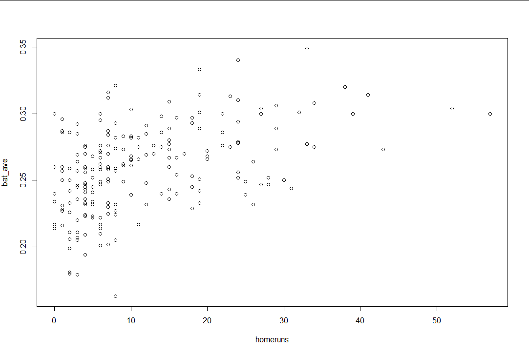
plot(baseball$homeruns,baseball$bat_ave,
     xlab = "homeruns",ylab = "bat_ave")

(2) Experimental results

2. Question 2

(1) Experimental code

# Two Paints Scatter Chart
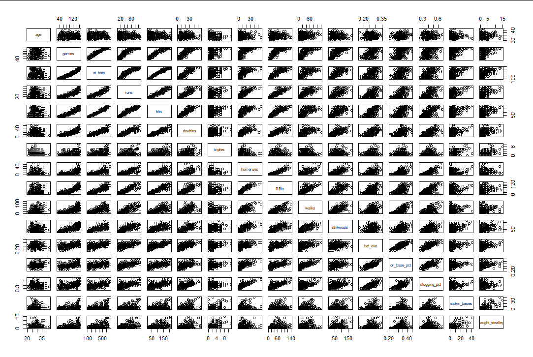
baseball1=baseball[,c(-1,-2,-4)]
pairs(baseball1)
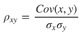
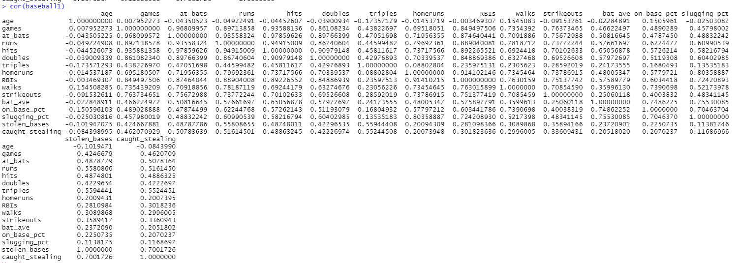
# Calculate correlation coefficient

(2) Principle analysis

(3) Experimental results

(4) Interpretation of results

The calculation of the clearance scatterplot and the linear correlation coefficient shows that:
game and at_bats,runs,hits,doubles,RBIs,walks, strikeouts have linear correlation
at_bats and runs,hits,doubles,RBIs have linear correlation
runs and hits,doubles,homeruns,RBIs have linear correlation
hits and doubles,RBIs have linear correlation
Linear correlation between doubles and RBIs
Horuns and RBIs have linear correlation
bat_ave and on_base_pct,slugging_pct has linear correlation
on_base_pct and slugging_pct has linear correlation

3. Question 3

(1) Experimental code

#Modeling
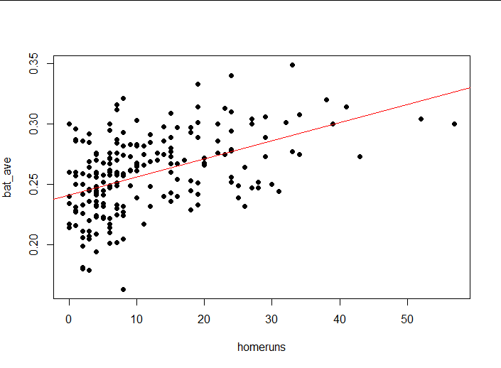
lm1<-lm(baseball$bat_ave~baseball$homeruns)
plot(bat_ave ~ homeruns,
     data = baseball,
     pch = 16,
     col = "black",
     ylab = "bat_ave")

abline(lm1, col = "red")#Draw a model on a scatterplot
# Note that this is the standardized residuals
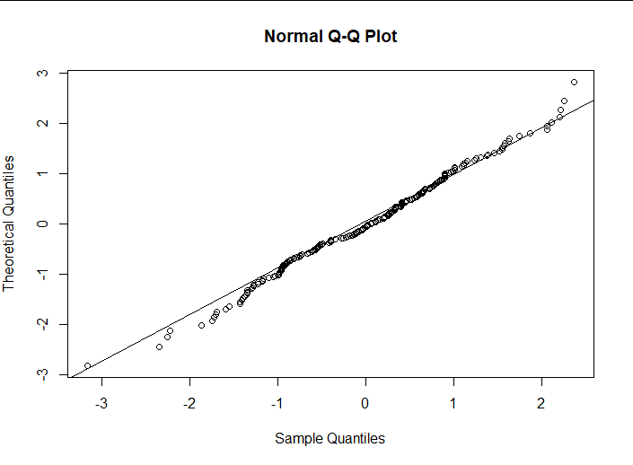
qqnorm(rstandard(lm1), datax = TRUE)
qqline(rstandard(lm1), datax = TRUE)

plot_ZP = function(ti) # Draw normal probability map
{
  n = length(ti)
  order = rank(ti)   #In ascending order, t(i) is the first order
  Pi = order/n #Cumulative probability
  plot(ti,Pi,xlab = "standard_residual",ylab = "Percentage")  #Draw normal probability map
  #Add Regression Line
  fm = lm(Pi~ti)
  abline(fm)
}
plot_ZP(rstandard(lm1))

(2) Principle analysis

(3) Experimental results

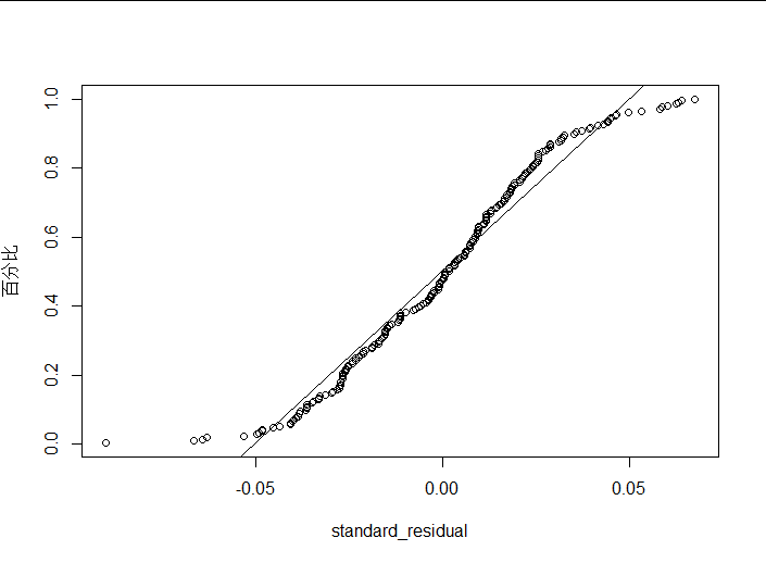
(4) Interpretation of results

I think residuals can be considered normal within an acceptable range

4. Question 4

(1) Experimental code

plot(lm1$fitted.values, lm1$residuals,pch = 16, col = "red",main = "
Residuals by Fitted Values",  ylab = "Residuals", xlab = "Fitted Values")
abline(0,0)

(2) Principle analysis

nothing

(3) Experimental results

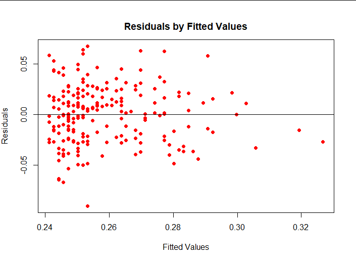
(4) Interpretation of results

From the results, you can see that the zero mean hypothesis is met, but others can clearly see that the distribution of residuals changes with the value of fitted values.

5. Question 5

(1) Experimental code

baseball$log_homeruns <- log(baseball$homeruns+1e-5)#Logarithm
lm2<-lm(baseball$bat_ave~baseball$log_homeruns)
plot(bat_ave ~ log_homeruns,
     data = baseball,
     pch = 16,
     col = "black",
     ylab = "bat_ave")

abline(lm2, col = "red")#Draw a model on a scatterplot

# Note that this is the standardized residuals
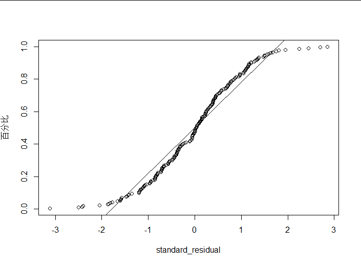
qqnorm(rstandard(lm2), datax = TRUE)
qqline(rstandard(lm2), datax = TRUE)
plot_ZP(rstandard(lm2))

(2) Principle analysis

nothing

(3) Experimental results

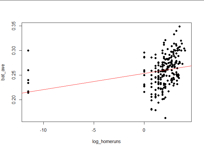
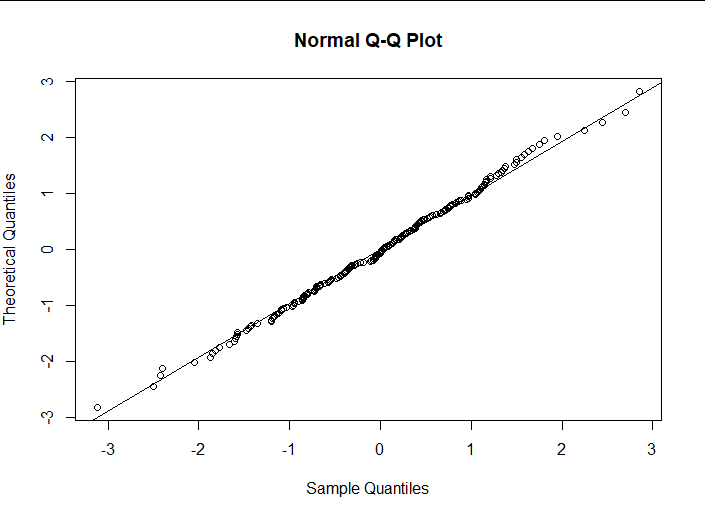
(4) Interpretation of results

Logarithms show that the distribution of standardized residuals is more normal.

6. Title 6

(1) Experimental code

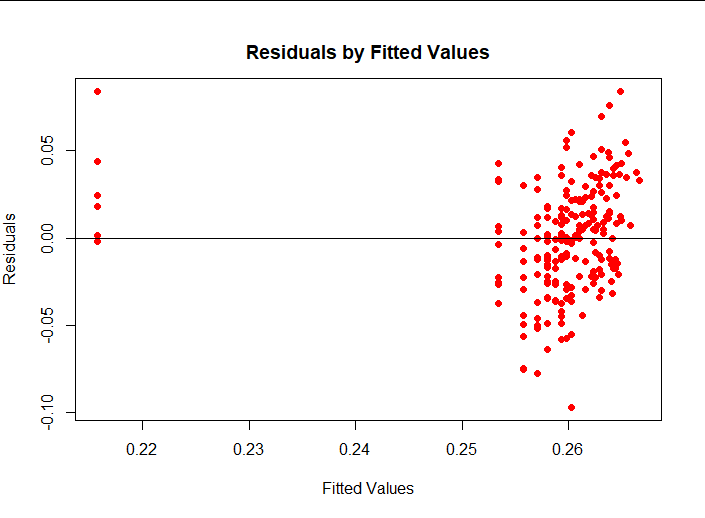
plot(lm2$fitted.values, lm2$residuals,pch = 16, col = "red",main = "
Residuals by Fitted Values",  ylab = "Residuals", xlab = "Fitted Values")
abline(0,0)

(2) Principle analysis

nothing

(3) Experimental results

(4) Interpretation of results

Without looking at the outliers, you can see that residual s satisfy the four assumptions in the book.

7. Topic 7

(1) Experimental code

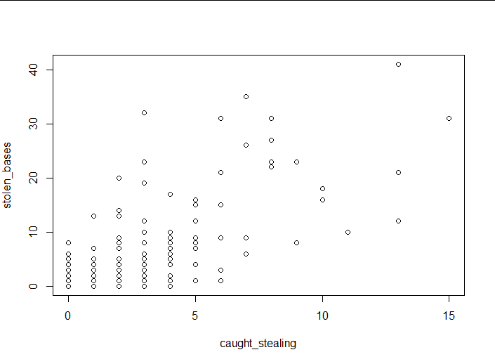
plot(baseball$caught_stealing,baseball$stolen_bases,
     xlab = "caught_stealing",ylab = "stolen_bases")

(2) Principle analysis

nothing

(3) Experimental results

(4) Interpretation of results

It can be seen that there is some correlation.

8. Question 8

(1) Experimental code

nothing

(2) Principle analysis

nothing

(3) Experimental results

nothing

(4) Interpretation of results

Some transformations are needed, because you can see from the scatterplot that there is a correlation between the two, but it's not obvious, and it's harder to see that there is a linear relationship.

9. Question 9

(1) Experimental code

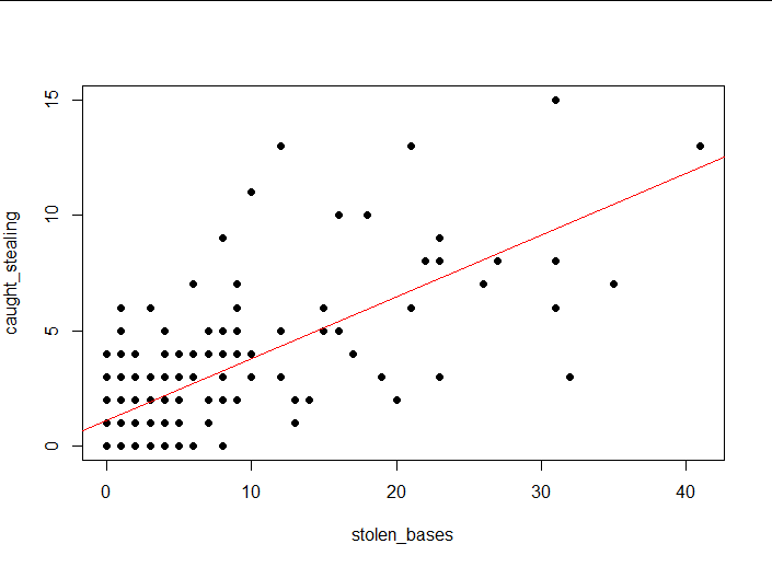
lm3<-lm(baseball$caught_stealing~baseball$stolen_bases)
plot(caught_stealing ~ stolen_bases,
     data = baseball,
     pch = 16,
     col = "black",
     ylab = "caught_stealing")

abline(lm3, col = "red")#Draw a model on a scatterplot

(2) Principle analysis

nothing

(3) Experimental results

(4) Interpretation of results

It does feel like there are some linear relationships.

10.Topic 10

(1) Experimental code

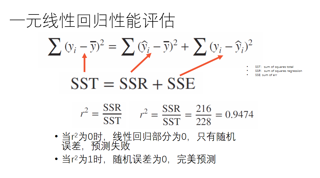
a1<-anova(lm3)
r2.1 <- a1$"Sum Sq"[1] / (a1$"Sum Sq"[1] +
                            a1$"Sum Sq"[2])

(2) Principle analysis

(3) Experimental results

(4) Interpretation of results

This r^2 value is not small, but it is not large enough.

11.11 Question 11

(1) Experimental code

nothing

(2) Principle analysis

nothing

(3) Experimental results

nothing

(4) Interpretation of results

Because only one observation variable is selected, it is easy to miss the explanatory variable.

Jobs for cereal datasets

1. Topic 1

(1) Experimental code

cereal <- read.csv("datasets/cereals.csv",stringsAsFactors=TRUE, header=TRUE)
plot(cereal$Sodium, cereal$Rating,pch = 16, col = "red",  ylab = "Rating", xlab = "Sodium")
lm1<-lm(cereal$Rating~cereal$Sodium)
standard_res=rstandard(lm1)
which(abs(standard_res)>2)

(2) Principle analysis

An outlier is considered if the absolute value of the standardized residuals exceeds 2

(3) Experimental results

(4) Interpretation of results

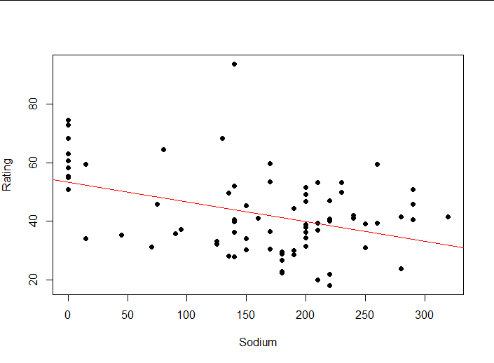
The fourth data is outliers.

2. Question 2

(1) Experimental code

plot(Rating ~ Sodium,
     data = cereal,
     pch = 16,
     col = "black",
     ylab = "Rating")

abline(lm1, col = "red")#Draw a model on a scatterplot

(2) Principle analysis

nothing

(3) Experimental results

(4) Interpretation of results

nothing

3. Question 3

(1) Experimental code

nothing

(2) Principle analysis

nothing

(3) Experimental results

(4) Interpretation of results

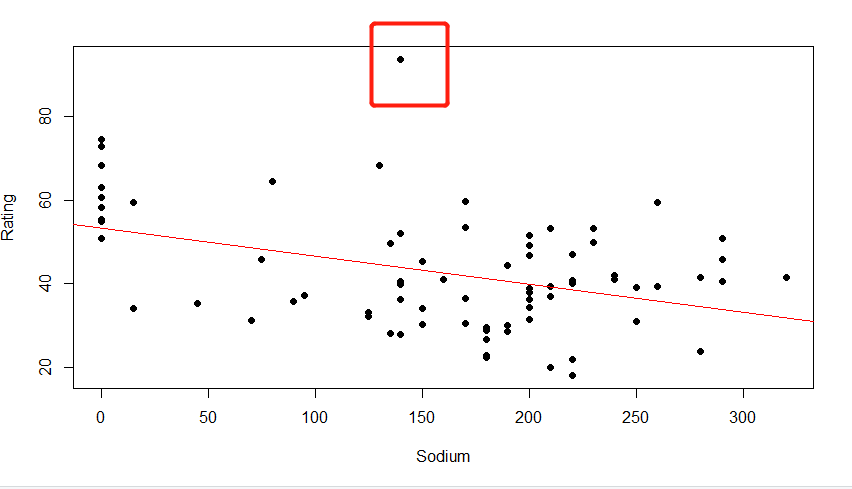
The slope and intercept do not differ much, indicating that an occasional outlier does not have much effect on linear regression

4. Question 4

(1) Experimental code

nothing

(2) Principle analysis

nothing

(3) Experimental results

(4) Interpretation of results

As shown in the red box in the figure above, outliers occur because the score is too high and the x-axis coordinates are still within the normal range, so the outlier causes the intercept value to change more than the slope.