2021SC@SDUSC

0. Preface

This blog post is mainly about the self attention mechanism of deep learning, qkv part and gradient in deep learning

1. Self attention mechanism of deep learning

1.1 basic concepts of self attention mechanism

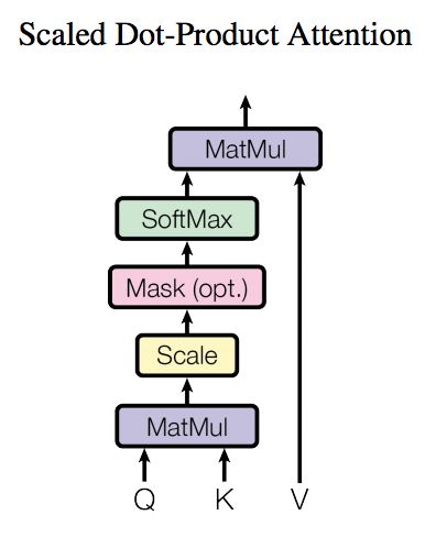
For the self attention mechanism, Q, K and V, that is, query, key and value, all come from the same input. First, calculate the point multiplication between Q and K, and then divide the result by a scale root dk, where dk is the latitude of a qurey and key vector. Then, the result is normalized to the probability distribution by Softmax operation, and then multiplied by matrix V to obtain the representation of weight summation. This operation can be expressed as
Attention can collect a set of qurey and key value pairs to the output, where qurey, keys, values and output are vectors, where the dimensions of query and keys are dk, and the dimensions of values are dv. The output is calculated as the weighted sum of values, and the weight assigned to each value is calculated by the similarity function between query and the corresponding key. This form of attention is called "scaled dot product attention".

1.2 qkv acquisition method

*

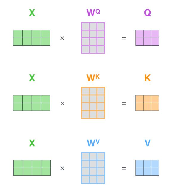
• Output operation to z
  

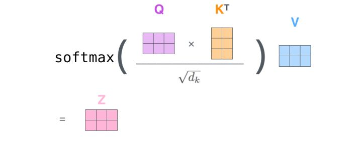
2.2 code analysis of self attention mechanism

2.2.1 data analysis

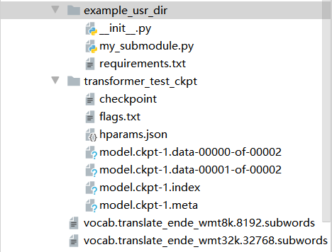
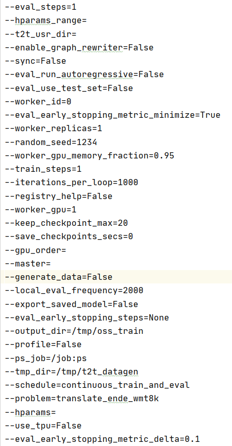
flags

2.2.2 partial code analysis

def real_env_step_increment(hparams):
  """Real env step increment."""
  return int(math.ceil(
      hparams.num_real_env_frames / hparams.epochs
  ))

Define real-world step increments

def setup_directories(base_dir, subdirs):
  """Setup directories."""
  base_dir = os.path.expanduser(base_dir)
  tf.gfile.MakeDirs(base_dir)
  all_dirs = {}
  for subdir in subdirs:
    if isinstance(subdir, six.string_types):
      subdir_tuple = (subdir,)
    else:
      subdir_tuple = subdir
    dir_name = os.path.join(base_dir, *subdir_tuple)
    tf.gfile.MakeDirs(dir_name)
    all_dirs[subdir] = dir_name
  return all_dirs

Set directory

def make_relative_timing_fn():
  start_time = time.time()
  def format_relative_time():
    time_delta = time.time() - start_time
    return str(datetime.timedelta(seconds=time_delta))
  def log_relative_time():
    tf.logging.info("Timing: %s", format_relative_time())
    return log_relative_time

Create a function that records the time since it was created.

def random_rollout_subsequences(rollouts, num_subsequences, subsequence_length):
  def choose_subsequence():
    rollout = random.choice(rollouts)
    try:
      from_index = random.randrange(len(rollout) - subsequence_length + 1)
    except ValueError:
      return choose_subsequence()
    return rollout[from_index:(from_index + subsequence_length)]
  return [choose_subsequence() for _ in range(num_subsequences)]

Select a random frame sequence of a given length from a set of rollout s
Train supervision

def train_supervised(problem, model_name, hparams, data_dir, output_dir,
                     train_steps, eval_steps, local_eval_frequency=None,
                     schedule="continuous_train_and_eval"):
  """Train supervised."""
  if local_eval_frequency is None:
    local_eval_frequency = FLAGS.local_eval_frequency

  exp_fn = trainer_lib.create_experiment_fn(
      model_name, problem, data_dir, train_steps, eval_steps,
      min_eval_frequency=local_eval_frequency
  )
  run_config = trainer_lib.create_run_config(model_name, model_dir=output_dir)
  exp = exp_fn(run_config, hparams)
  getattr(exp, schedule)()

Set hparams override in the unresolved parameter list:

def set_hparams_from_args(args):
  """Set hparams overrides from unparsed args list."""
  if not args:
    return
  hp_prefix = "--hp_"
  tf.logging.info("Found unparsed command-line arguments. Checking if any "
                  "start with %s and interpreting those as hparams "
                  "settings.", hp_prefix)

  pairs = []
  i = 0
  while i < len(args):
    arg = args[i]
    if arg.startswith(hp_prefix):
      pairs.append((arg[len(hp_prefix):], args[i+1]))
      i += 2
    else:
      tf.logging.warn("Found unknown flag: %s", arg)
      i += 1

  as_hparams = ",".join(["%s=%s" % (key, val) for key, val in pairs])
  if FLAGS.hparams:
    as_hparams = "," + as_hparams
  FLAGS.hparams += as_hparams

2. Full connection layer

2.1 definition and function of full connection layer

• fully connected layers (FC) play the role of "Classifier" in the whole convolutional neural network. The convolution layer, activation function and pooling layer map the original data to the hidden layer feature space, while the full connection layer plays a role to learn "In practical use, the fully connected layer can be realized by convolution operation: for the previous layer, the fully connected fully connected layer can be transformed into a convolution with a convolution core of 1 * 1; while the former layer is a convolution layer, the fully connected layer can be transformed into a global convolution with a convolution core of hw, which is the height and width of the convolution result of the previous layer respectively. The most important and core of the fully connected layer is the weight of the matrix, which we pass After in-depth learning, the weight of this layer is repeatedly trained to obtain the best weight matrix W.
• Sometimes it is impossible to solve the nonlinear problem with only one layer of fully connected layers, but if there are more than two layers of fully connected layers, the nonlinear problem can be solved well.

2.2 partial code analysis

A fully connected NN layer.
N_units: number of neurons in int layer
Input_shape: the expected input shape of the tuple layer.
For dense layers, a single number specifying the number of input features. Must be specified if it is the first layer in the network.

class Dense(Layer):
    """A fully-connected NN layer.
    Parameters:
    -----------
    n_units: int
        The number of neurons in the layer.
    input_shape: tuple
        The expected input shape of the layer. For dense layers a single digit specifying
        the number of features of the input. Must be specified if it is the first layer in
        the network.
    """
    def __init__(self, n_units, input_shape=None):
        self.layer_input = None
        self.input_shape = input_shape
        self.n_units = n_units
        self.trainable = True
        self.W = None
        self.w0 = None

    def initialize(self, optimizer):
        # Initialize the weights
        limit = 1 / math.sqrt(self.input_shape[0])
        self.W  = np.random.uniform(-limit, limit, (self.input_shape[0], self.n_units))
        self.w0 = np.zeros((1, self.n_units))
        # Weight optimizers
        self.W_opt  = copy.copy(optimizer)
        self.w0_opt = copy.copy(optimizer)

    def parameters(self):
        return np.prod(self.W.shape) + np.prod(self.w0.shape)

    def forward_pass(self, X, training=True):
        self.layer_input = X
        return X.dot(self.W) + self.w0

    def backward_pass(self, accum_grad):
        # Save weights used during forwards pass
        W = self.W

        if self.trainable:
            # Calculate gradient w.r.t layer weights
            grad_w = self.layer_input.T.dot(accum_grad)
            grad_w0 = np.sum(accum_grad, axis=0, keepdims=True)

            # Update the layer weights
            self.W = self.W_opt.update(self.W, grad_w)
            self.w0 = self.w0_opt.update(self.w0, grad_w0)

        # Return accumulated gradient for next layer
        # Calculated based on the weights used during the forward pass
        accum_grad = accum_grad.dot(W.T)
        return accum_grad

    def output_shape(self):
        return (self.n_units, )

3. Summary

• Self attention is the basis of transformer, bert and gpt. Mastering self attention is the only way to learn deep learning algorithm
• Deep neural network models generally take the full connection layer as the last layer to be used as a classifier. The full connection layer is actually matrix multiplication. W e have only one parameter to learn.