In the first two articles, we have introduced the autoregressive model pixelcnn and how to deal with multidimensional input data. In this article, we will focus on one of the biggest limitations of pixelcnn (i.e. blind spots) and how to improve it to repair it.
In the first two articles, we introduced the concept of generating model PixelCNN and studied the working principle of color PixelCNN. Pixel CNN is a generation model for learning pixel probability distribution. The intensity of pixels in the future will be determined by the previous pixels. In previous articles, we implemented two PixelCNN and noticed that the performance was not excellent. We also mentioned that one of the ways to improve the performance of the model is to fix the blind spot problem. In this article, we will introduce the concept of blind spot, discuss how pixel CNN is affected, and implement a solution - gated pixel CNN.
blind spot
Pixel CNN learns the conditional distribution of all pixels in the image and uses this information for prediction. PixelCNN will learn the distribution of pixels from left to right and from top to bottom, Generally, A mask is used to ensure that the "future" pixels (i.e. the pixels to the right or below the pixel being predicted) cannot be used for the prediction of A given pixel. As shown in figure A below, the mask clears the pixels "after" the currently predicted pixel (which corresponds to the pixel in the center of the mask). However, this operation results in not all "past" All pixels will be used to calculate new points, and the lost information will produce blind spots.
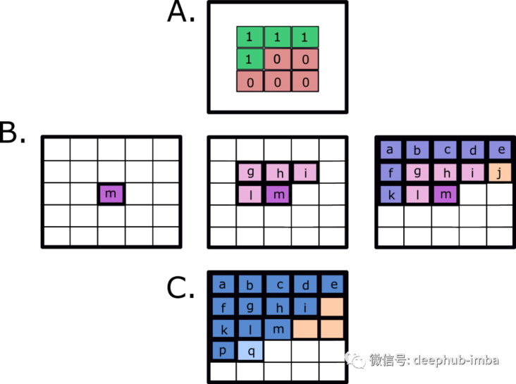
To understand the blind spot problem, let's look at figure B. In Figure B, the dark pink dot (m) is the pixel we want to predict because it is located in the center of the filter. If we use a 3x3 mask (A. above), pixel m depends on l, G, h, i. On the other hand, these pixels depend on the previous pixels. For example, pixel g depends on f, a, B, C, and pixel I depends on H, C, d, e. From the above figure B, we can also see that although it appears before pixel m, pixel j is never considered to calculate the prediction of M. Similarly, if we want to predict q, j, n and o, we will never consider it (orange part of C above). Therefore, not all previous pixels will affect the prediction, which is called the blind spot problem.
We will first look at the implementation of pixelcnn and how blind spots will affect the results. The following code snippet shows the pixelcnn implementation mask using Tensorflow 2.0.
class MaskedConv2D(keras.layers.Layer):
    """Convolutional layers with masks.
    Convolutional layers with simple implementation of masks type A and B for
    autoregressive models.
    Arguments:
    mask_type: one of `"A"` or `"B".`
    filters: Integer, the dimensionality of the output space
        (i.e. the number of output filters in the convolution).
    kernel_size: An integer or tuple/list of 2 integers, specifying the
        height and width of the 2D convolution window.
        Can be a single integer to specify the same value for
        all spatial dimensions.
    strides: An integer or tuple/list of 2 integers,
        specifying the strides of the convolution along the height and width.
        Can be a single integer to specify the same value for
        all spatial dimensions.
        Specifying any stride value != 1 is incompatible with specifying
        any `dilation_rate` value != 1.
    padding: one of `"valid"` or `"same"` (case-insensitive).
    kernel_initializer: Initializer for the `kernel` weights matrix.
    bias_initializer: Initializer for the bias vector.
    """

    def __init__(self,
                 mask_type,
                 filters,
                 kernel_size,
                 strides=1,
                 padding='same',
                 kernel_initializer='glorot_uniform',
                 bias_initializer='zeros'):
        super(MaskedConv2D, self).__init__()

        assert mask_type in {'A', 'B'}
        self.mask_type = mask_type

        self.filters = filters
        self.kernel_size = kernel_size
        self.strides = strides
        self.padding = padding.upper()
        self.kernel_initializer = initializers.get(kernel_initializer)
        self.bias_initializer = initializers.get(bias_initializer)

    def build(self, input_shape):
        self.kernel = self.add_weight('kernel',
                                      shape=(self.kernel_size,
                                             self.kernel_size,
                                             int(input_shape[-1]),
                                             self.filters),
                                      initializer=self.kernel_initializer,
                                      trainable=True)

        self.bias = self.add_weight('bias',
                                    shape=(self.filters,),
                                    initializer=self.bias_initializer,
                                    trainable=True)

        center = self.kernel_size // 2

        mask = np.ones(self.kernel.shape, dtype=np.float64)
        mask[center, center + (self.mask_type == 'B'):, :, :] = 0.
        mask[center + 1:, :, :, :] = 0.

        self.mask = tf.constant(mask, dtype=tf.float64, name='mask')

    def call(self, input):
        masked_kernel = tf.math.multiply(self.mask, self.kernel)
        x = nn.conv2d(input,
                      masked_kernel,
                      strides=[1, self.strides, self.strides, 1],
                      padding=self.padding)
        x = nn.bias_add(x, self.bias)
        return x
Looking at the receiving domain of the original pixel CNN (marked with yellow in Figure 2 below), we can see the blind spot and how it propagates on different layers. In the second part of this article, we will use the improved PixelCNN, gated PixelCNN, which introduces a new mechanism to avoid the generation of blind spots.
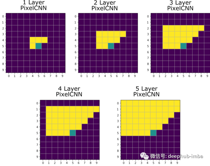
Figure 2: visualization of blind spot area on pixel CNN
Gated PixelCNN
In order to solve these problems, van den Oord et al. (2016) introduced gated pixel CNN. Gated PixelCNN is different from PixelCNN in two main aspects:
- It solves the blind spot problem
- The performance of the model is improved by using gated convolution
How does gated pixel CNN solve the blind spot problem
This new model solves the blind spot problem by integrating the volume into two parts: vertical and horizontal stack. Let's see how vertical and horizontal stacks work.

Figure 3: vertical (green) and horizontal stacks (blue)
In the vertical stack, the goal is to process the context information of all rows before the current row. The method to ensure that all previous information is used and causality is maintained (the currently predicted pixel should not know the information on its right) is to move the center of the mask upward to the row above the predicted pixel respectively. As shown in Figure 3, the center is a light green pixel (m), but the information collected by the vertical stack is not used to predict it, but to predict the pixel (r) of the row below it.
Using the vertical stack alone creates a blind spot on the left side of the black prediction pixel (m). To avoid this, the information collected by the vertical stack is combined with the information from the horizontal stack (p-q in blue in Fig. 3) to predict all pixels to the left of the pixel (m) to be predicted. The combination of horizontal and vertical stacks solves two problems:
(1) The information to the right of the predicted pixel is not used,
(2) Because we consider it as a block, there is no blind spot.
The original paper realized the vertical stack by convolution of receptive field with 2x3. In this article, we do this by using 3x3 convolution and masking the last line. In the horizontal stack, the convolution layer associates the predicted value with the data from the current analysis pixel row. This can be achieved using 1x3 convolution, so that future pixels can be shielded to ensure the causality condition of the autoregressive model. Similar to PixelCNN, we implement type A mask (for the first layer) and type B mask (for subsequent layers).
The following code snippet shows the mask implemented using the Tensorflow 2.0 framework.
class MaskedConv2D(keras.layers.Layer):
    """Convolutional layers with masks.

    Convolutional layers with simple implementation of masks type A and B for
    autoregressive models.

    Arguments:
    mask_type: one of `"A"` or `"B".`
    filters: Integer, the dimensionality of the output space
        (i.e. the number of output filters in the convolution).
    kernel_size: An integer or tuple/list of 2 integers, specifying the
        height and width of the 2D convolution window.
        Can be a single integer to specify the same value for
        all spatial dimensions.
    strides: An integer or tuple/list of 2 integers,
        specifying the strides of the convolution along the height and width.
        Can be a single integer to specify the same value for
        all spatial dimensions.
        Specifying any stride value != 1 is incompatible with specifying
        any `dilation_rate` value != 1.
    padding: one of `"valid"` or `"same"` (case-insensitive).
    kernel_initializer: Initializer for the `kernel` weights matrix.
    bias_initializer: Initializer for the bias vector.
    """

    def __init__(self,
                 mask_type,
                 filters,
                 kernel_size,
                 strides=1,
                 padding='same',
                 kernel_initializer='glorot_uniform',
                 bias_initializer='zeros'):
        super(MaskedConv2D, self).__init__()

        assert mask_type in {'A', 'B', 'V'}
        self.mask_type = mask_type

        self.filters = filters
        self.kernel_size = kernel_size
        self.strides = strides
        self.padding = padding.upper()
        self.kernel_initializer = initializers.get(kernel_initializer)
        self.bias_initializer = initializers.get(bias_initializer)

    def build(self, input_shape):
        kernel_h = self.kernel_size
        kernel_w = self.kernel_size
        self.kernel = self.add_weight('kernel',
                                      shape=(self.kernel_size,
                                             self.kernel_size,
                                             int(input_shape[-1]),
                                             self.filters),
                                      initializer=self.kernel_initializer,
                                      trainable=True)

        self.bias = self.add_weight('bias',
                                    shape=(self.filters,),
                                    initializer=self.bias_initializer,
                                    trainable=True)
        mask = np.ones(self.kernel.shape, dtype=np.float64)

        # Get centre of the filter for even or odd dimensions
        if kernel_h % 2 != 0:
            center_h = kernel_h // 2
        else:
            center_h = (kernel_h - 1) // 2

        if kernel_w % 2 != 0:
            center_w = kernel_w // 2
        else:
            center_w = (kernel_w - 1) // 2

        if self.mask_type == 'V':
            mask[center_h + 1:, :, :, :] = 0.
        else:
            mask[:center_h, :, :] = 0.
            mask[center_h, center_w + (self.mask_type == 'B'):, :, :] = 0.
            mask[center_h + 1:, :, :] = 0.

        self.mask = tf.constant(mask, dtype=tf.float64, name='mask')

    def call(self, input):
        masked_kernel = tf.math.multiply(self.mask, self.kernel)
        x = nn.conv2d(input,
                      masked_kernel,
                      strides=[1, self.strides, self.strides, 1],
                      padding=self.padding)
        x = nn.bias_add(x, self.bias)
        return x
By adding the characteristic graphs of the two stacks to the whole network, we get an autoregressive model with consistent receptive fields and no blind spots (Fig. 4).
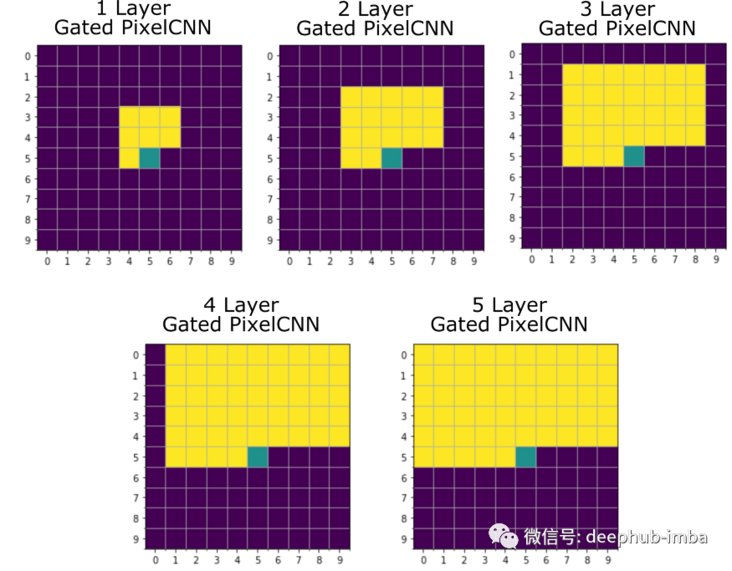
Figure 4: visualization of receptive field of gated pixel CNN. We note that using a combination of vertical and horizontal stacks, we can avoid the blind spot problem observed in the initial version of pixel CNN (compare Figure 2).
Door control activation unit (or door control block)
The second major improvement from the original PixelCNN to the gated CNN is the introduction of gated blocks and multiplication units (in the form of LSTM gates). Therefore, instead of using ReLU between mask convolutions like the original PixelCNN, the Gated PixelCNN uses a gated activation unit to simulate more complex interactions between features. This gated activation unit uses sigmoid (as a forgetting gate) and tanh (as a real activation). In the original paper, the author believes that this may be one of the reasons why PixelRNN (using LSTM) is better than PixelCNN, because they can better capture past pixels through loops - they can remember past information. Therefore, Gated PixelCNN adds and uses the following:

σ Is sigmoid, k is the number of layers, ⊙ is the element product, * is the convolution operator, and W is the weight from the previous layer. With this formula, we can introduce the single layer in pixel CNN in more detail.
Single layer block in gated pixel CNN
Stack and gate are the basic blocks of gated pixel CNN (Figure 5 below). But how are they connected and how will the information be processed? We will decompose it into four processing steps, which will be discussed in the following session.
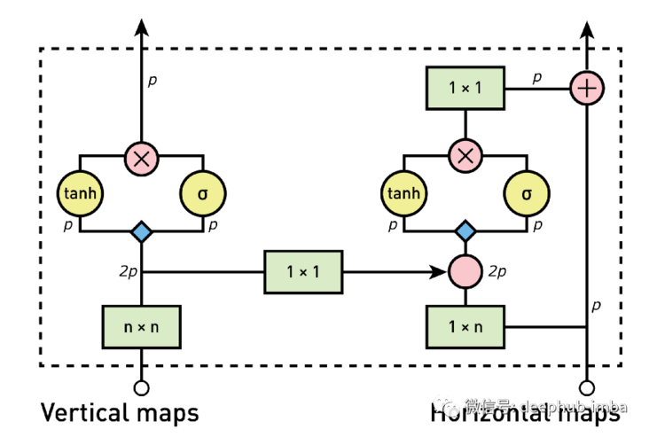
Figure 5: overview of the gated pixel CNN architecture (image from the original paper). Colors represent different operations (i.e., green: convolution; red: element multiplication and addition; blue: convolution with weight
1. Calculate vertical stack characteristic diagram
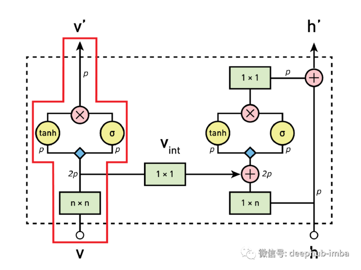
As a first step, the input from the vertical stack is processed by 3x3 convolution layer and vertical mask. The generated feature map is then gated to activate the unit and input into the vertical stack of the next block.
2. Send vertical map to horizontal stack

For autoregressive models, it is necessary to combine the information of vertical and horizontal stacks. For this purpose, the vertical stack in each block is also used as one of the inputs to the horizontal layer. Since the center of each convolution step of the vertical stack corresponds to the analyzed pixels, we cannot add only the vertical information, which will break the causality condition of the autoregressive model, because it will allow the information of future pixels to be used to predict the values in the horizontal stack. This is the case in the second figure in Figure 8A below, The pixel to the right (or future) of the black pixel is used to predict it. For this reason, you need to use fill and crop to move it down before providing vertical information to the horizontal stack (Figure 8B). By zero filling the image and cropping the bottom of the image, you can ensure the causal relationship between vertical and horizontal stacks. We will delve into more details of how cropping works in a future article, so don't worry if its details are not completely clear
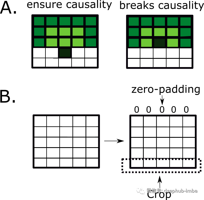
Figure 8: how to ensure the causal relationship between pixels
3. Calculation horizontal characteristic diagram
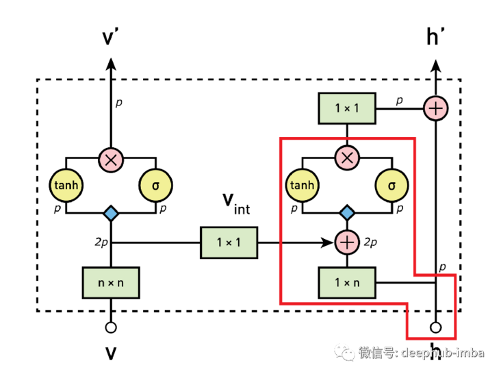
In this step, the characteristic map of horizontal convolution is processed. In fact, first, sum the feature mapping output from vertical convolution to horizontal convolution. The output of this combination has an ideal receiving format, which takes into account the information of all previous pixels, and then through the gated activation unit.
4. Calculate the residual connection on the horizontal stack
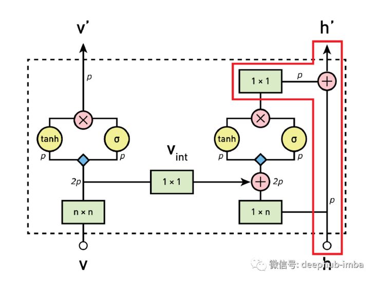
In this last step, if the block is not the first block of the network, the residual connection is used to merge the output of the previous step (after 1x1 convolution), and then sent to the horizontal stack of the next block. Skip this step if it is the first block of the network.
The code for using Tensorflow 2 is as follows:
class GatedBlock(tf.keras.Model):
    """ Gated block that compose Gated PixelCNN."""

    def __init__(self, mask_type, filters, kernel_size):
        super(GatedBlock, self).__init__(name='')

        self.mask_type = mask_type
        self.vertical_conv = MaskedConv2D(mask_type='V',
                                          filters=2 * filters,
                                          kernel_size=kernel_size)

        self.horizontal_conv = MaskedConv2D(mask_type=mask_type,
                                            filters=2 * filters,
                                            kernel_size=kernel_size)

        self.padding = keras.layers.ZeroPadding2D(padding=((1, 0), 0))
        self.cropping = keras.layers.Cropping2D(cropping=((0, 1), 0))

        self.v_to_h_conv = keras.layers.Conv2D(filters=2 * filters, kernel_size=1)

        self.horizontal_output = keras.layers.Conv2D(filters=filters, kernel_size=1)

    def _gate(self, x):
        tanh_preactivation, sigmoid_preactivation = tf.split(x, 2, axis=-1)
        return tf.nn.tanh(tanh_preactivation) * tf.nn.sigmoid(sigmoid_preactivation)

    def call(self, input_tensor):
        v = input_tensor[0]
        h = input_tensor[1]

        vertical_preactivation = self.vertical_conv(v)

        # Shifting vertical stack feature map down before feed into horizontal stack to
        # ensure causality
        v_to_h = self.padding(vertical_preactivation)
        v_to_h = self.cropping(v_to_h)
        v_to_h = self.v_to_h_conv(v_to_h)

        horizontal_preactivation = self.horizontal_conv(h)

        v_out = self._gate(vertical_preactivation)

        horizontal_preactivation = horizontal_preactivation + v_to_h
        h_activated = self._gate(horizontal_preactivation)
        h_activated = self.horizontal_output(h_activated)

        if self.mask_type == 'A':
            h_out = h_activated
        elif self.mask_type == 'B':
            h_out = h + h_activated

        return v_out, h_out
In conclusion, the gating block is used to solve the blind spot problem in the receiving domain and improve the performance of the model.
Comparison of results
In the original paper, pixel CNN uses the following architecture: the first layer is a mask convolution (type A) with 7x7 filter. Then 15 residual blocks are used. Each block uses a combination of 3x3 layer convolution layer of mask class B and standard 1x1 convolution layer to process data. Between each convolution layer, ReLU is used for activation. Finally, some residual links are included.
So we trained a pixel CNN and a gated pixel CNN, and compared the results below.
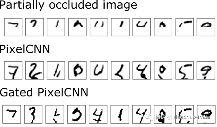
When comparing the MNIST predictions of PixelCNN and Gated PixelCNN (above), we did not find much improvement in MNIST. Some previously revised forecasts are now incorrectly predicted. This does not mean that PixelCNN is not performing well. In the next blog post, we will discuss PixelCNN + + with gating, so please continue to pay attention!
Gated pixel CNN paper address: https://arxiv.org/abs/1606.05328
By Walter Hugo Lopez Pinaya, Pedro F. da Costa, and Jessica Dafflon