1. Introduction of BP algorithm

1.1 Background

Enlightened by the neural network in the human brain, computer simulation of the neural network in the human brain is used to realize machine learning technology of artificial intelligence. The bp algorithm is the most successful neural network algorithm to date. The bp algorithm can be used in multi-layer forward neural network.

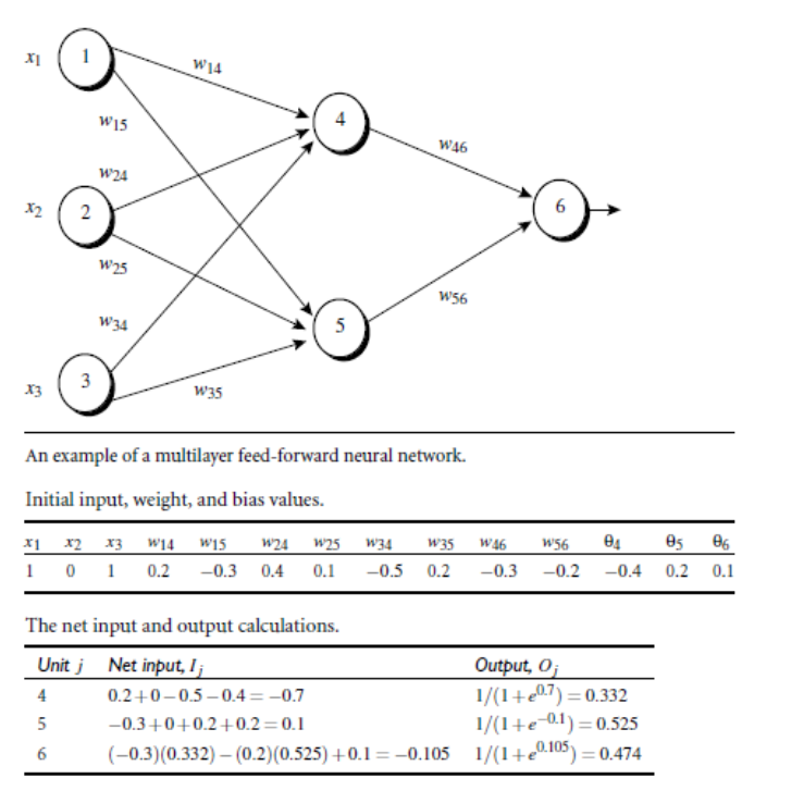
1.2 Multilayer Feed-Forward Neural Network

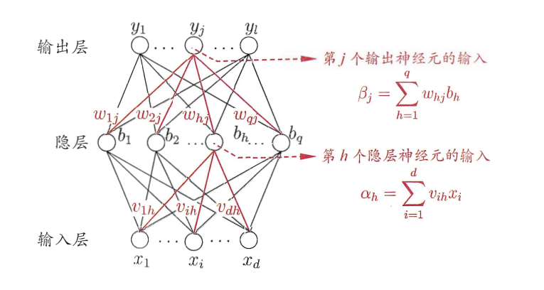
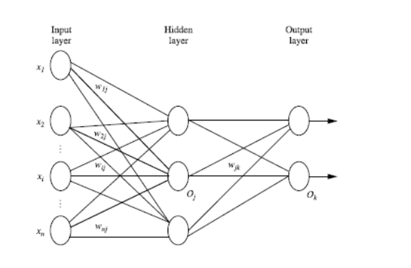
Multilayer Feedforward Neural Networks Each layer of neurons is fully interconnected to the next layer, and there is no homologous or cross-layer connection between neurons.
A multilayer feed-forward neural network consists of the following components:
Input layer, hidden layers, output layers

Introduction to neural networks:

1. Each layer consists of neurons
2. The input layer is passed in by the instance eigenvector of the training set
3. The weights of the connected nodes are passed to the next layer, and the output of the first layer is the input of the next layer
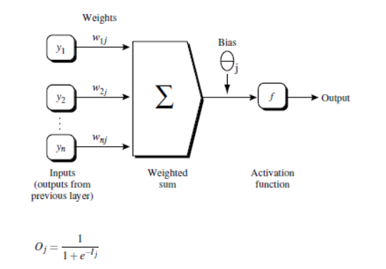
4. The input values of each neuron are the cumulative sum of the output and corresponding weights of all the neurons connected to it by the upper layer, and the output values of each layer are the cumulative and added thresholds, which are then transformed according to the equation.
5. The number of hidden layers can be arbitrary, one for input and one for output.
6. The output layer does not count as the number of layers of the neural network. There are any number of hidden layers. All the neural networks can simulate any calculation equation.

Design of 1.3 Neural Network Structure

Neural networks are mostly used to solve classification problems. Before training data with neural networks, the number of layers of the network and the number of neurons in each layer must be determined. To speed up the learning process of neural networks when datasets are passed into the input layer, data is usually standardized between 0-1
Determination of the number of neurons in the input layer:
Determined by the type of data set, the number of neurons in the input layer is usually equal to the number of classes. For example, watermelon color A may have three values of black, Turquoise and light white, then the number of neurons in the input layer can be set to 3. If the input data is black (A = black), then the number of neurons representing black will be 1, and the other two neurons will be 0.
Determining the number of neurons in the output layer:
For classification problems, if there are two classes, they can be represented by one output unit (0 and 1 represent two classes respectively). If there are two extra classes, each class is represented by one output unit
Determining the number of neurons in the hidden layer:
There are no clear rules to design how many hidden layers it is best to have. Experiments and improvements are made based on experimental tests, errors, and accuracy.

1.4 bp algorithm process

Overall, the bp algorithm mainly processes the training set instances through iteration, the main step is to update the values of each neuron layer in the positive direction, then compare the errors between the predicted value (output layer value) and the true value of the neural network in the reverse direction to minimize the errors and update the weights of each connection and the thresholds of each neuron
Algorithm Introduction

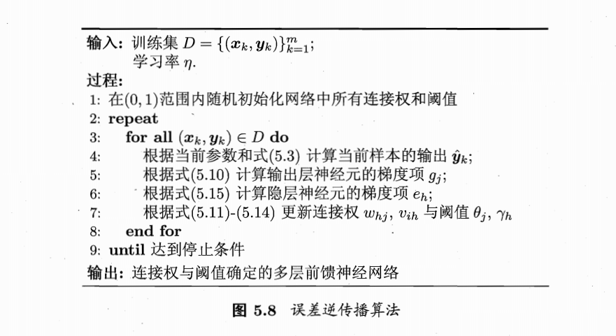
1.4.1 Initialization

Initialization weights and thresholds

1.4.2 Forward update of neuron values

Steps:

1. Assign each instance of training data to the input layer
2. The input values of hidden layer neurons are the cumulative sum of input layer values and corresponding weights
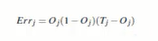
3. Hidden layer neurons sum input values and thresholds and convert them to output values by a function.
4. The input values of output layer neurons are the cumulative sum of hidden layer output values and corresponding weights
5. Output layer neurons sum input values and thresholds and convert them to output values by a function.

1.4.3 Reverse updating of weights and thresholds

Update weights and thresholds inversely from the output layer to the output layer based on the difference between the value of the output layer and the true value
Steps:

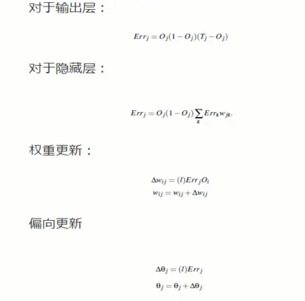
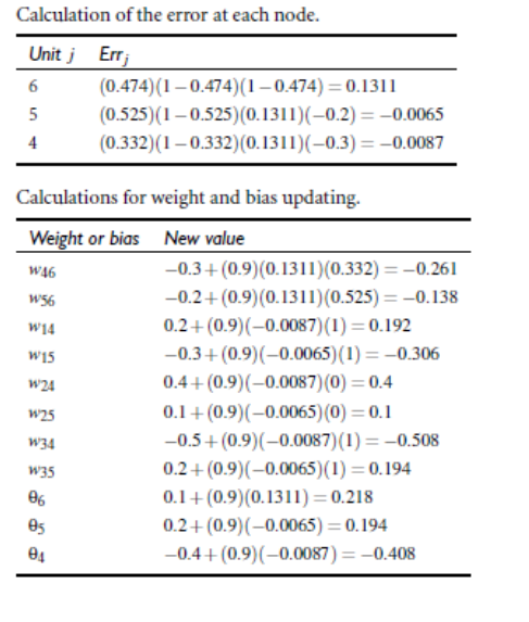
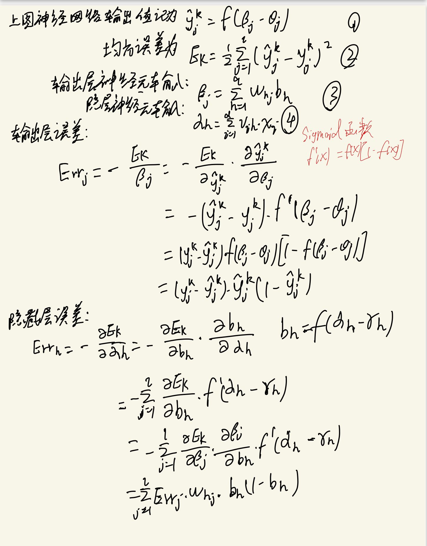
1. Output layer error:
   
   That is, output layer error = predicted value* (1-predicted value)* (true value-predicted value)

2. Hidden layer error:
   
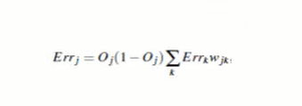
   Hidden Layer Error = Layer Output* (1-Layer Output) (Next Layer Error Corresponds to Weight Cumulative Sum)

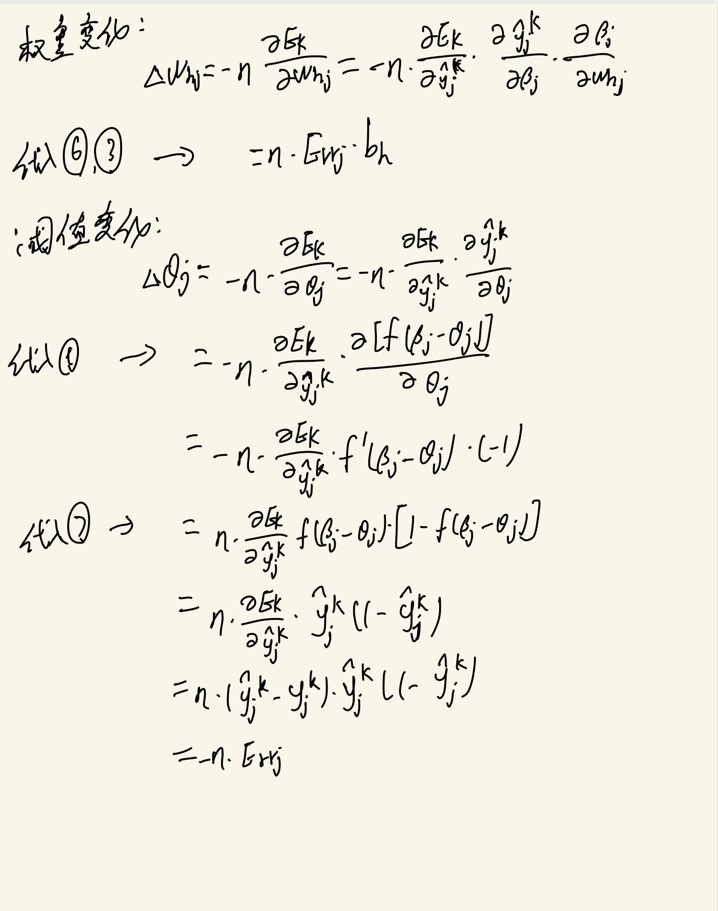
3. Weight update:
   
   Weight = Current Weight + Learning Rate Next Error Current Output

4. Threshold update:
   
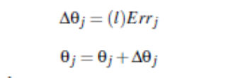
   That is, bias = current bias + learning rate * current layer error

5. Output layer neurons sum input values and thresholds and convert them to output values by a function.

1.4.4 algorithm stop

The algorithm stopping conditions can be determined based on the actual model training. Generally, there are three stopping conditions

1. Weight updates are below a threshold
2. The prediction error rate is below a threshold
3. Reach a preset number of cycles

1.5 bp algorithm example

2. Deduction of BP algorithm theory

This section takes the contents and formulas in Chapter V of Zhou Zhihua's Watermelon Book as the basis and reference to deduce the theory.

3. Examples of BP algorithm codes

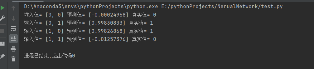
Let's take a very general example of a neural network, which implements the value of a prediction XOR operation with a training set of
[
([0 0],0)
([0 1],1)
([1 0],1)
([1 1],0)
]

import numpy as np

#Defining hyperbolic functions
def tanh(x):
    return np.tanh(x)

#Hyperbolic function derivative
def tanh_deriv(x):
    return 1.0 - np.tanh(x) * np.tanh(x)

#Define logical functions
def logistic(x):
    return 1 / (1 + np.exp(-x))

#Define logical function derivatives
def logistic_derivative(x):
    return logistic(x) * (1 - logistic(x))


class NeuralNetwork:
    def __init__(self, layers, activation='logistic'):
        if activation == 'logistic':
            self.activation = logistic#self.activation is a logical function
            self.activation_deriv = logistic_derivative
        elif activation == 'tanh':
            self.activation = tanh
            self.activation_deriv = tanh_deriv

        self.weights = []#Define weights
        for i in range(1, len(layers) - 1):#Weight Initialization Random Assignment
            self.weights.append((2 * np.random.random((layers[i - 1] + 1, layers[i] + 1)) - 1) * 0.25)
            self.weights.append((2 * np.random.random((layers[i] + 1, layers[i + 1])) - 1) * 0.25)
        print(self.weights)
    def fit(self, X, y, learning_rate=0.2, epochs=10000):
        '''
        X:input data
        y:Prediction Marker
        learning_rate:learning rate
        epochs:Set number of algorithm executions
        '''
        X = np.atleast_2d(X) # Convert to an m*n matrix
        print("Input Dataset\n",X)
        temp = np.ones([X.shape[0], X.shape[1] + 1])  #Initialize an m*(n+1) matrix X.shape=(4,2)

        print("Initialization Matrix m*n\n",temp)
        temp[:, 0:-1] = X  # Assignment of offsets
        X = temp
        print("Offset\n",X)
        y = np.array(y)
        print(np.random.randint(X.shape[0]))
        for k in range(epochs):
            i = np.random.randint(X.shape[0])  #Random number from 0 to m-1
            a = [X[i]]                         #Assign the row to i

            for l in range(len(self.weights)):  # Update the value of each neuron forward
                sum_weights=np.dot(a[l], self.weights[l])
                a.append(self.activation(sum_weights))
            error = y[i] - a[-1]  #The difference between the true value and the predicted value
            deltas = [error * self.activation_deriv(a[-1])]  # Errors in calculating the output layer correspond to the output layer calculation formula

            # Staring backprobagation
            for l in range(len(a) - 2, 0, -1):  # we need to begin at the second to last layer
                # Compute the updated error (i,e, deltas) for each node going from top layer to input layer
                deltas.append(deltas[-1].dot(self.weights[l].T) * self.activation_deriv(a[l]))  #Compute Hidden Layer Error Corresponds to Hidden Layer Calculation Formula
            deltas.reverse()
            for i in range(len(self.weights)):
                layer = np.atleast_2d(a[i])   #
                delta = np.atleast_2d(deltas[i])
                self.weights[i] += learning_rate * layer.T.dot(delta)  #Weight Update Formula

    def predict(self, x):
        x = np.array(x)
        temp = np.ones(x.shape[0] + 1)
        temp[0:-1] = x
        a = temp
        for l in range(0, len(self.weights)):
            a = self.activation(np.dot(a, self.weights[l]))
        return a


nn=NeuralNetwork([2,2,1],'tanh')
x=np.array([[0,0],[0,1],[1,0],[1,1]])
y=np.array([0,1,1,0])
nn.fit(x,y)
for index,data in enumerate([[0,0],[0,1],[1,0],[1,1]]):
    print("Input Value=",data,"predicted value=",nn.predict(data),"True Value=",y[index])

The results are as follows: