introduction
With the growth of business volume, the cache schemes used generally go through the following steps: 1) query DB directly without cache; 2) Data synchronization + Redis; 3) Multi level cache has three stages.
In the first stage, direct DB query can only be used in small traffic scenarios. With the increase of QPS, cache needs to be introduced to reduce the pressure on DB.
In the second stage, the data will be synchronized to redis through the message queue, and redis will be updated synchronously when the data changes. Redis will be queried directly during business query. If redis has no data, go to the DB. The disadvantage of this scheme is that if redis fails, the cache avalanche will directly call the traffic to the DB, which may further hang up the DB, resulting in business accidents.
In the third stage, redis cache is used as the second level cache, and a layer of local cache is added to it. Redis is checked when the local cache misses, and DB is checked when redis misses. The advantage of using local cache is that it is not affected by external systems and has good stability. The disadvantage is that it is impossible to update in real time like the distributed cache, and due to the limited memory, it is necessary to set the cache size and formulate the cache elimination strategy, so there will be a hit rate problem.
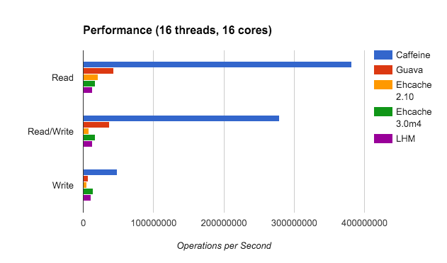
This article will mainly introduce a local cache solution - Caffeine (a high-performance, high hit rate, near optimal local cache, known as "new generation cache" or "king of modern cache". Starting from Spring 5, Caffeine will replace Guava Cache as the default cache component of Spring).
Cache way
Local cache is to cache data in the memory space of the same process, and data reading and writing are completed in the same process; The distributed cache is an independently deployed process and is generally deployed on different machines from the application process, so the data transmission of distributed cache data reading and writing operations needs to be completed through the network. Compared with the distributed cache, the local cache has fast access speed, but it does not support large amount of data storage, it is difficult to ensure the data consistency of each node during data update, and the data is lost with the restart of the application process.
Cache is generally a data structure of key value pairs, corresponding to HashMap and ConcurrentHashMap in Java. Because HashMap is thread unsafe (concurrent put will loop), CHM is generally used as the local cache. A simple local cache can be implemented using CHM, but due to the limited memory, it is only suitable for scenes with small amount of data. As the amount of data increases, the memory will expand infinitely, so you need to use the elimination strategy to eliminate the unused cache.
Common elimination algorithms include FIFO (First In First Out), LRU (Least Recently Used), LFU (Least Frequently Used), etc. FIFO is more in line with the conventional thinking, first come first serve, which is also common in the design of the operating system. However, when used in the cache, there will be the problem that the first high-frequency data will be eliminated and the last low-frequency data will be retained, resulting in low cache hit rate. LRU is the least used recently. If a data has not been accessed in the recent period of time, it is also very unlikely to be accessed next. When the space is full, the least accessed data will be eliminated first. The problem here is that if a large amount of data is accessed one minute ago and there is no access within one minute, the hot data will be eliminated. LFU has the least frequency of use recently. If a data is rarely used in the recent period of time, the probability of its use in the future is also very small. The difference from LRU is that LRU is based on access time and LFU is based on access frequency. LFU uses additional space to record the usage frequency of each data, and then selects the lowest frequency for elimination, which solves the problem that LRU cannot process the time period. The hit rate of these three algorithms is better than one, but the implementation cost is also higher than one. In the actual implementation, the middle LRU is generally selected.
In practical use, the appeal elimination algorithm still has the following problems: a) serious lock competition; b) Expiration time is not supported; c) Automatic refresh is not supported. To solve these problems, Guava Cache came into being. Guava Cache and java1 Similar to CHM in 7, using segmented locking reduces lock granularity and increases concurrency. Guava Cache provides two expiration strategies: expiration after reading and expiration after writing. Expired elements do not expire immediately, but are processed during read-write operations to avoid global locking during background thread scanning. Automatic refresh is to judge whether the refresh conditions are met during query. In addition, Guava Cache has features such as recycling by reference, removing listeners, elegant Api and so on.
Guava Cache is powerful and easy to use, but its essence is still the encapsulation of LRU algorithm, which has inherent defects in cache hit rate. Caffeine proposes a more efficient cache structure similar to the LFU admission strategy, TinyLFU and its variant W-TinyLFU, and draws lessons from the design experience of Guava Cache to obtain a new generation of local cache with powerful function and better performance.
Amazing algorithm
introduction
The most intuitive reason why caching can work is that there is a certain degree of locality in data access in many fields of computer science. It is a common way to capture the locality of data through probability distribution. However, in many fields, the probability distribution is quite inclined, that is, only a small number of objects are accessed by high frequency. Moreover, in many scenarios, the access pattern and its corresponding probability distribution change with time, that is, it has time locality.
If the probability distribution corresponding to the data access mode does not change with time, the highest cache hit rate can be obtained by using LFU. However, LFU has two limitations: first, it needs to maintain a large number of complex metadata (the space used to maintain which elements should be written to the cache and which should be eliminated is called cached metadata); Second, in the actual scene, the access frequency changes fundamentally with the passage of time. For example, after a hot play has been popular for a period of time, it may be ignored. For the appeal problem, there are many variants of LFU, mainly using aging mechanism or limited size sampling window. The purpose is to limit the size of metadata and focus caching and elimination decisions on the recently popular elements. Window LFU (WLFU) is one of them.
In most cases, the newly accessed data is always directly inserted into the cache, and the cache designer only focuses on the eviction strategy, because it is considered impractical to maintain the metadata of objects that are not currently in the cache. In the existing implementation of LFU, only the frequency histogram of elements in the cache is maintained. This LFU is called in memory LFU. The corresponding is Perfect LFU (PLFU), which maintains the frequency histogram of all visited objects. The effect is the best, but the maintenance cost is prohibitive.
LRU is a very common algorithm used to replace LFU. LRU eliminates the least recently used elements, which will be more efficient than LFU and automatically adapt to sudden access requests; However, LRU based caching usually requires more space overhead to achieve the same cache hit rate as LFU.
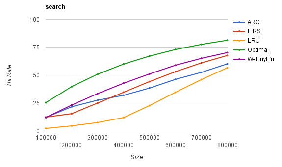
In view of the above background and problems, Ben Manes et al TinyLFU: A Highly Efficient Cache Admission Policy The effectiveness of a cache structure / algorithm similar to LFU admission strategy is clarified, and the rationality of Caffeine cache component is demonstrated theoretically and experimentally. Its specific contributions are as follows:
- A cache structure is proposed, which can be inserted only when the admission strategy thinks that replacing it into the cache will improve the cache hit rate;
- TinyLFU, a new data structure with high space utilization, is proposed, which can approximately replace the data statistics part of LFU in the scenario of large traffic;
- Through formal proof and simulation, it is proved that the Freq ranking obtained by TinyLFU is almost similar to the real access frequency ranking;
- TinyLFU is implemented in Caffeine project in the form of Optimization: W-TinyLFU;
- Compared with other cache management strategies, including ARC, LIRC and so on.
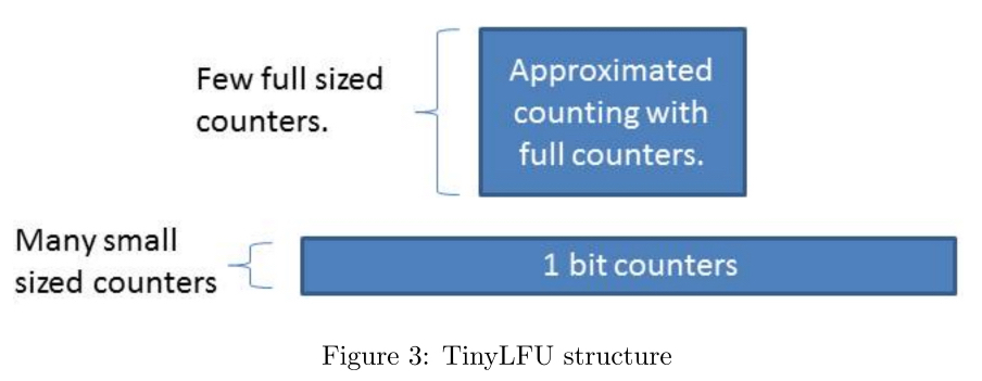
TinyLFU structure
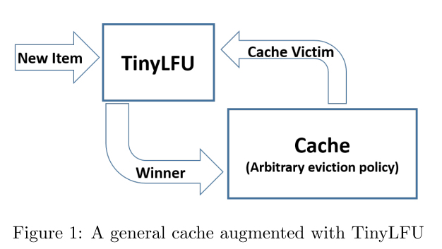
The structure of TinyLFU is shown in the figure. For the elements determined to be eliminated by the cache expulsion strategy, TinyLFU determines whether to replace them according to the principle of whether replacing the old elements with new elements into the cache will help to improve the cache hit rate. Therefore, TinyLFU needs to maintain a large historical access frequency statistics, which is very expensive. Therefore, TinyLFU uses some efficient approximate calculation techniques to approximate these statistics
approximate calculation
Bloom Filter is a binary vector data structure proposed by Howard Bloom in 1970. It has good space and time efficiency (insertion / query time is constant) and is used to detect whether an element is a member of the set. If the detection result is yes, the element is not necessarily in the set; However, if the detection result is no, the element must not be in the collection. Since the Bloom Filter does not need to store the element itself, it is also suitable for scenes with strict confidentiality requirements. The disadvantage is that the miscalculation rate increases with the increase of the number of elements. Another point is that elements cannot be deleted, because the hash result of multiple elements may be the same bit, and deleting a bit may affect the detection of multiple elements.
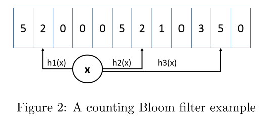
Counting Bloom Filter (CBF) adds an additional counter to each bit of the standard bloom filter. When inserting elements, add 1 to the corresponding k (number of hash functions) counters respectively, and subtract 1 when deleting elements
Minimum increment CBF is an enhanced counting bloom filter, which supports two methods: addition and estimation. The evaluation method first calculates k different hash values for the key, reads the corresponding counters with the hash value as the index, and takes the minimum value of these counters as the return value. The addition method is similar to this. After reading K counters, only the smallest counter is increased. As shown in the figure below, three hash functions correspond to three counters. When {2,2,5} is read, the addition operation will only increase 2 to 3 and 5, which remains unchanged, so as to make a better estimation of high-frequency elements, because the counters of high-frequency elements are unlikely to be increased by many low-frequency elements. The minimum increment CBF does not support attenuation, but experience shows that this method can reduce the error of high-frequency counting.
Cm sketch is another popular approximate counting scheme, which makes a trade-off between accuracy and space, and trades for smaller space occupation and faster speed with less accuracy loss. Moreover, the spatial optimization and aging mechanism introduced later can be directly applied to CM sketch
Freshness mechanism
At present, the known way to maintain the freshness of approximate sketch (A sketch of a large amount of data is a small data structure that lets you calculate or approximate certain characteristics of the original data) is to use an ordered list containing m different sketches for sliding sampling, and the new elements are inserted into the first sketch, After a certain number of inserts, the last sketch is cleared and moved to the list header to discard the old elements. This method has two disadvantages: a) in order to evaluate the frequency of an element, m different approximate sketches need to be read, resulting in many memory accesses and hash calculations; b) Because the same elements are stored in M different sketches and more counters are allocated to each element, the space overhead increases.
For these two problems, a Reset method is proposed to maintain the freshness of sketch. The Reset method increments a counter every time an element is added to the approximate sketch. Once the counter reaches the sampling size w, it divides all counters in the approximate sketch by 2. This direct division method has two advantages: first, there is no additional space overhead, because its memory overhead is a single counter occupying Log(W) bits; Secondly, the accuracy of high-frequency elements is increased. The disadvantage of this scheme is that it needs to traverse all counters and divide them by 2. However, the division by 2 operation can be implemented efficiently in hardware with shift register, and shift and mask can be used to perform this operation on multiple small counters at the same time in software implementation. Therefore, the sharing complexity of divide by two operations is constant and can be applied to a variety of application scenarios.
Space optimization
There are two ways of space optimization: one is to reduce the size of each counter in sketch, and the other is to reduce the total number of counters allocated in sketch.
Small counter
The implementation of approximate sketch generally uses Long counter. If a sketch wants to accommodate w requests, it requires the maximum value of the counter to reach W, and each counter needs to occupy Log(W) bits. This overhead is very large. Considering that the frequency histogram only needs to know whether the elements to be eliminated are more popular than the currently accessed elements, without knowing the exact order of all items in the cache, and for the cache of size C, all elements with an access frequency of more than 1/C should belong to the cache (it is reasonable to assume that the total number of elements accessed is greater than C), so for a given sampling size w, The upper limit of the counter can be set to W/C
Gatekeeper mechanism
In many scenarios, especially in the long tail scenario, inactive elements account for a large proportion. If the number of accesses to each element is counted, most counters are assigned to elements that are unlikely to occur many times. In order to further reduce the number of counters, Doorkeeper mechanism is used to avoid assigning counters to tail objects.
Doorkeeper is a conventional bloom filter placed before the approximate counting strategy. When accessing an element, first judge whether the element is in doorkeeper. If not, write the element into doorkeeper, otherwise write it into the main structure. When querying elements, doorkeeper and the main structure are calculated together. If in doorkeeper, the number of elements in the main structure is increased by 1, and if not, the number of elements in the main structure is returned directly. When the Reset operation is performed, all counters in the main structure will be halved and the doorkeeper will be cleared at the same time. In this way, you can clear all the information of the first counter (also increase the truncation error by 1).
In terms of memory, although Doorkeeper requires additional space, it makes the main structure smaller by limiting the number of elements written into the main structure. Especially in the long tail scenario, most of the long tail elements only occupy the 1-bit counter in Doorkeeper. Therefore, this optimization will greatly reduce the memory overhead of TinyLFU. The structure of Doorkeeper in TinyLFU is shown in the figure.
W-TinyLFU optimization
TinyLFU looks good in most scenes, but for scenes with sparse burst traffic, when the new burst traffic cannot accumulate enough times to keep it in the cache, these elements will be eliminated and repeated miss will occur. This problem is remedied by introducing W-TinyLFU structure when TinyLFU is integrated into Caffeine.
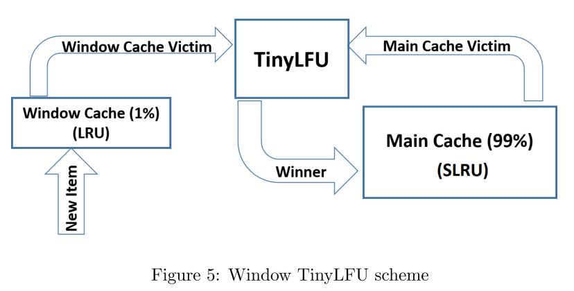
The structure of W-TinyLFU is shown in the figure. It is composed of two cache units. The main cache uses SLRU expulsion policy and TinyLFU admission policy, and the window cache only uses LRU expulsion policy without admission policy. Select the hotspots in the non-static cache (80% of the hotspots in the Ru A1 and A2) and allocate them to the hotspots in the non-static cache (80% of the hotspots in the Ru A1 and A2). Any incoming element is always allowed to enter the window cache. The eliminated elements of the window cache have the opportunity to enter the main cache. If they are accepted by the main cache, the eliminated W-TinyLFU is the eliminated person of the main cache, otherwise it is the eliminated person of the window cache.
In Caffeine, the window cache accounts for 1% of the total cache and the main cache accounts for 99%. The motivation behind W-TinyLFU is to handle the work of LFU in the way of TinyLFU, and still make use of the advantages of LRU in dealing with sudden traffic. Because 99% of the cache is allocated to the main cache, the impact on the performance of LFU work is negligible. On the other hand, in the scenario applicable to LRU, W-TinyLFU is better than TinyLFU. Generally speaking, W-TinyLFU is the first choice in various business scenarios, so the complexity brought by introducing it into Caffeine is acceptable.
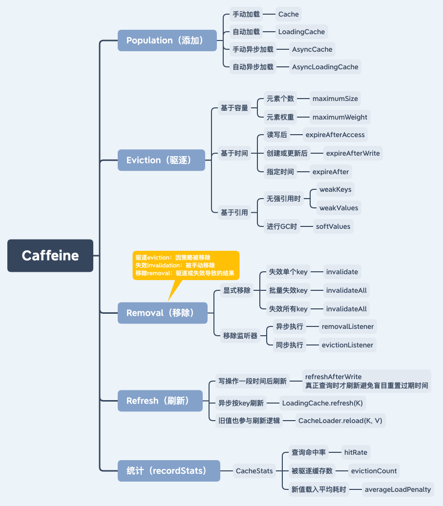
Elegant implementation
The main functions of Caffeine are shown in the figure. It supports manual / automatic, synchronous / asynchronous cache loading methods, expulsion strategy based on capacity, time and reference, listener removal, cache hit rate, average loading time and other statistical indicators.
Introduction to use
Caffeine supports four cache loading strategies: manual loading, automatic loading, manual asynchronous loading and automatic asynchronous loading. The usage gestures of various caches are as follows.
/** Manual loading */
Cache<Key, Graph> cache = Caffeine.newBuilder()
    .expireAfterWrite(10, TimeUnit.MINUTES)
    .maximumSize(10_000)
    .build();

Graph graph = cache.getIfPresent(key);
graph = cache.get(key, k -> createExpensiveGraph(key));
cache.put(key, graph);
cache.invalidate(key);

/** Automatic loading */
LoadingCache<Key, Graph> cache = Caffeine.newBuilder()
    .maximumSize(10_000)
    .expireAfterWrite(10, TimeUnit.MINUTES)
    .build(key -> createExpensiveGraph(key));

Graph graph = cache.get(key);
Map<Key, Graph> graphs = cache.getAll(keys);

/** Manual asynchronous loading */
AsyncCache<Key, Graph> cache = Caffeine.newBuilder()
    .expireAfterWrite(10, TimeUnit.MINUTES)
    .maximumSize(10_000)
    .buildAsync();

CompletableFuture<Graph> graph = cache.getIfPresent(key);
graph = cache.get(key, k -> createExpensiveGraph(key));
cache.put(key, graph);
cache.synchronous().invalidate(key);

/** Automatic asynchronous loading */
AsyncLoadingCache<Key, Graph> cache = Caffeine.newBuilder()
    .maximumSize(10_000)
    .expireAfterWrite(10, TimeUnit.MINUTES)
    // You can choose to encapsulate a synchronous operation asynchronously to generate cache elements
    .buildAsync(key -> createExpensiveGraph(key));
    // You can also choose to build an asynchronous cache element operation and return a future
    .buildAsync((key, executor) -> createExpensiveGraphAsync(key, executor));

// Find the cache element. If it does not exist, it will be generated asynchronously
CompletableFuture<Graph> graph = cache.get(key);
// Batch search cache elements. If they do not exist, they will be generated asynchronously
CompletableFuture<Map<Key, Graph>> graphs = cache.getAll(keys);
Overall design
Sequential access queue
Access order queue is a two-way linked list, which arranges the elements in all hashtables in order. An element can find and operate its adjacent elements in the queue from the HashMap within the time complexity of O(1). Access order is defined as the order in which elements in the cache are created, updated, or accessed. The least recently used element will be at the head of the queue, and the most recently used element will be at the end of the queue. This helps the implementation of capacity-based eviction policy (maximumSize) and idle time based expiration policy (expireAfterAccess). The problem here is that each access changes the queue, so it can not be achieved through efficient concurrent operations.
Sequential write queue
The write order is defined as the order in which the elements in the cache are created and updated. Similar to the access queue, the operation of writing to the queue is also based on the time complexity of O(1). This queue provides help for the implementation of a lifetime based eviction strategy (expireAfterWrite).
Layered time wheel
Hierarchical time wheel is a priority queue with time as priority, which is realized by hash and two-way linked list. Its operation is also O(1) time complexity. This queue provides assistance for the implementation of a specified time-based eviction policy (expire after (expire)).
Read buffer
A typical cache implementation locks each operation so that the elements of each access queue can be safely sorted. An alternative is to add each reordered operation to the buffer for batch operation. This can be used as a pre write log for the page replacement policy. When the buffer is full, it will try to acquire the lock and hang. If the lock is held, the thread will return immediately.
The read buffer is a striped ring buffer. The design of ribbon is to reduce the resource competition between threads. A thread corresponds to a ribbon through hash. Ring buffer is a fixed length array that provides efficient performance and minimizes GC overhead. The specific number of ring queues can be dynamically adjusted according to the competition prediction algorithm.
Write buffer
Similar to read buffering, write buffering is used to replay write events. The events in the read buffer are mainly to optimize the hit rate of the expulsion strategy, so a certain degree of loss is allowed. However, write buffering does not allow data loss, so it must be implemented as an efficient bounded queue. Since the contents of the write buffer must be emptied every time the write buffer is filled, the capacity of the write buffer is usually empty or very small.
The write buffer is implemented by a ring array that can be expanded to the maximum size. When the size of the array is adjusted, the memory will be allocated directly to generate a new array. The pre array will point to the new array so that consumers can access it, which allows the old array to be released directly after access. This blocking mechanism allows the buffer to have a smaller initial size, lower read-write cost and generate less garbage. When the buffer is full and cannot be expanded, the producer of the buffer will try to spin and trigger the maintenance operation, and return to the executable state after a short time. In this way, the write priority of the thread can be determined by the write priority of the consumer.
Lock sharing
Traditional caching locks each operation, while Caffeine allocates the locking cost to each thread through batch processing. In this way, the side effects caused by locking will be shared equally by each thread to avoid the performance overhead caused by locking competition. The maintenance operation will be distributed to the configured thread pool for execution. When the task is rejected or the calling thread execution policy is specified, the user thread can also perform the maintenance operation.
One advantage of batch processing is that due to the exclusivity of locks, only one thread will process the data in the buffer at the same time. This will make the buffer implementation of consumption model based on multi producer / single consumer more efficient. This will also make better use of the advantages of CPU cache to better adapt to hardware characteristics.
Element state transition
When the cache is not protected by an exclusive lock, operations against the cache may be replayed in the wrong order. Under the condition of concurrent contention, a create read update delete sequential operation may not write to the cache in the correct order. If you want to ensure the correct order, you may need coarser grained locks, resulting in performance degradation.
Like typical concurrent data structures, Caffeine uses atomic state transition to solve this problem. A cache element has three states: survival, retirement and death. The survival status refers to the existence of an element in the Hash table and the access / write queue at the same time. When an element is removed from the Hash table, its state will also change to retirement and need to be removed from the queue. When it is also removed from the queue, the state of an element is considered dead and recycled in the GC.
Relaxed reads and writes
Caffeine has put a lot of effort into making full use of volatile operations. Memory barrier It provides a hardware perspective instead of thinking about volatile reading and writing from the language level. There is potential for better performance by understanding which barriers are established and their impact on hardware and data visibility.
When performing exclusive access under a lock, Caffeine uses relaxed reads because the visibility of data can be obtained through the memory barrier of the lock. This is acceptable when data contention cannot be avoided (such as checking whether the element expires when reading to simulate cache loss).
Caffeine uses relaxed writes in a similar way. When an element is written exclusively in the locked state, the write can be carried back on the memory barrier released when unlocking. This can also be used to support solving the write partial order problem, such as updating the timestamp when reading a data.
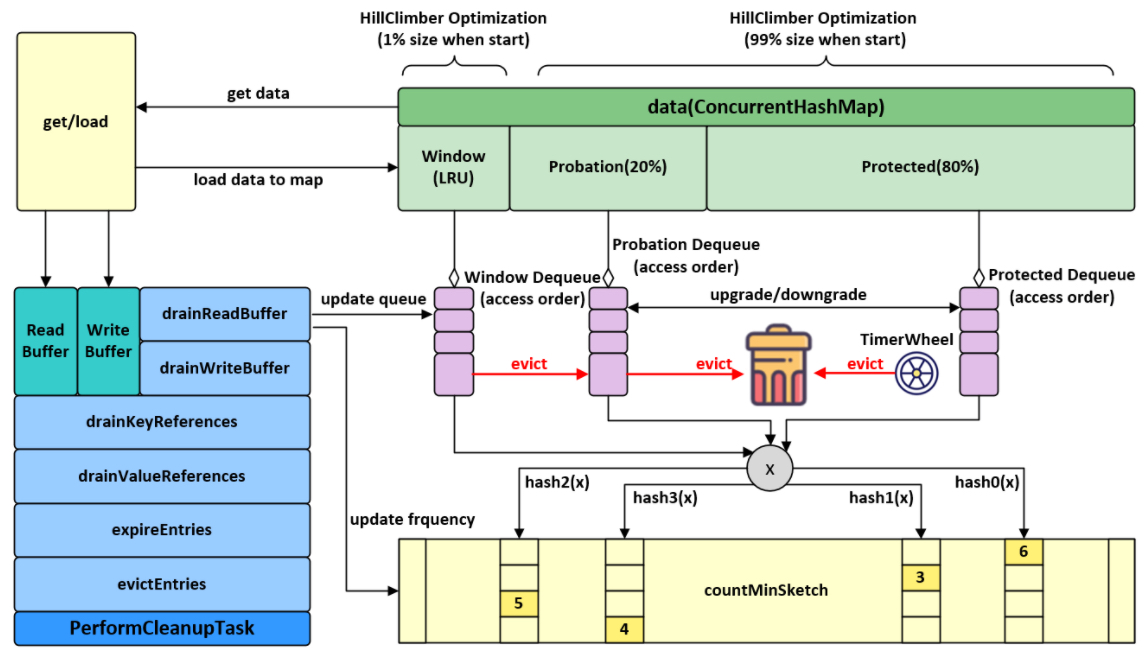
Expulsion strategy
Caffeine use Window TinyLfu The strategy provides almost optimal hit rate. The access queue is divided into two parts: the TinyLfu policy will expel the selected elements from the access window of the cache to the main space of the cache. TinyLfu will compare the access frequency between the victims in the window and the victims in the main space, and choose to retain the elements that have been accessed more frequently before. The frequency will be stored in CountMinSketch through 4 bits, which will occupy 8 bytes for each element to calculate the frequency. These designs allow the cache to expel the elements in the cache with O(1) time complexity based on access frequency and proximity at minimal cost.
Adaptability
The size of the admission window and the size of the main space will be dynamically adjusted based on the workload characteristics of the cache. The window will be larger when it is closer, and smaller when it is closer to the frequency. Caffeine uses the hill clipping algorithm to adjust the sampling hit rate and configure it to the best balance state.
Fast processing mode
When the size of the cache does not exceed 50% of the total capacity and the eviction strategy is not used, the sketch used to record the frequency will not be initialized to reduce the memory overhead, because the cache may be loaded artificially with a high threshold. When there are no other feature requirements, the access will not be recorded to avoid competition on the read buffer and replay the access events on the read buffer.
HashDoS protection
When the hash values between key s are the same, or the hash reaches the same location, this kind of hash conflict may lead to performance degradation. The hash table solves this problem by demoting the linked list to a red black tree.
One attack against TinyLFU is to artificially increase the estimated frequency of elements under the expulsion strategy by using hash conflict. This will cause all subsequent incoming elements to be rejected by the frequency filter, resulting in cache invalidation. One solution is to add a small amount of jitter to make the final result uncertain. This can be achieved by randomly enrolling about 1% of rejected candidates.
code generation
Cache has many different configurations, and the relevant fields are meaningful only when using a subset of specific functions. If all fields exist by default, it will lead to a waste of memory overhead of the cache and each element in the cache. Using code generation will reduce the memory overhead at runtime at the cost of storing larger binaries on disk.
This technology has the potential of algorithm optimization. Perhaps when constructing, the user can specify the most suitable feature according to usage. A mobile application may need a higher concurrency rate, while the server may need a higher hit rate under a certain memory overhead. It may not be necessary to constantly try to choose the best balance among all usages, but can be selected by driving algorithms.
Encapsulated hash map
The cache adds the required features by encapsulating it on the ConcurrentHashMap. The concurrency algorithm of cache and hash table is very complex. By separating the two, we can more easily apply the advantages of hash table design, and avoid the problems caused by coarser granularity lock covering the whole table and expulsion.
The cost of this approach is additional runtime overhead. These fields can be inline directly to the elements in the table, rather than wrapping to contain additional metadata. The lack of wrappers can provide a fast path for a single table operation (such as lambdas) rather than multiple map calls and short-lived object instances.
Source code analysis
Take an actual business scenario as an example. When a user clicks on a product when shopping on pinduoduo, he needs to display the name and Logo information of the store to which the product belongs. These are relatively stable information that will not change frequently. Due to the large volume of C-end users and the large number of people browsing goods per second, if these traffic directly reaches the database, the database may be hung up. Therefore, consider putting it into the cache in advance and fetching it from the cache when necessary. The code fragment of implementing such a query interface with Caffeine is as follows:
// Define an automatically loaded cache: it can hold up to 10000 stores and will automatically expire 30 hours after writing to the cache
LoadingCache<QueryMallBasicRequest, MallVO> mallBasicLocalCache = Caffeine.newBuilder()
            .initialCapacity(10_000)
            .maximumSize(10_000)
            .expireAfterWrite(Duration.ofHours(30))
            .recordStats(CatStatsCounter::new)
            .build(this::queryMallBasicInfo);

// Query the basic information of a store
MallVO mallVO = mallBasicLocalCache.get(request);
The visual expression of what the get() method does here is that if there is a value in the local cache, it will be returned directly. If there is no value, it will be set in the cache and returned after finding the value through the specified queryMallBasicInfo method. In fact, the logic behind it is much more complex. We start from the get method to track what Caffeine does behind it, so as to implement the above algorithm principle and framework design into the specific code implementation.
Class diagram
Check the class diagram under cache package. The solid blue line indicates inheritance and the dotted green line indicates interface implementation.
- LocalCache
The middle part is the two implementations of the LocalCache interface: BoundedLocalCache bounded cache and unbounded LocalCache unbounded cache.
LocalCache inherits and extends ConcurrentMap. As the framework of the whole Caffeine project, it provides thread safety and atomic guarantee.
Under BoundedLocalCache, there are four subclasses WS, SI, SS and wi (W stands for WeakKeys, I stands for InfirmValues, the first S stands for StrongKeys, and the second S stands for StrongValues). Under each of these four subclasses, there are seven subclasses. Subclasses generate subclasses, and finally there is a big lump. These capitalized classes are automatically generated by javapool. For the builder mode, combine the features available to the user into corresponding classes in advance. When the user defines caffeine After the builder, the corresponding generated classes are loaded directly according to the defined feature combination to improve the performance. For the corresponding code, please refer to the LocalCacheFactory#newBoundedLocalCache method.
Here's why there are 7 subclasses under each of the 4 subclasses. The optional features supported by Caffeine are as follows. The first is the most important reference types of key and value. Here, value defines four types. In fact, generateLocalCaches only uses Strong and Infirm. Therefore, the key value combination generates four subclasses. Each subclass has to traverse other features. In addition to the references of key and value, there are seven other features, Therefore, there are 7 subclasses under each. If you want to understand the code generation logic, you can download the source code of github and see the code in the javapool package. For a simple understanding, you can refer to the LocalCacheFactoryGenerator#getFeatures method.
- Node
At the bottom left is the node part, which is an element / entry in the cache, including key, value, weight, access and write metadata. Node is an abstract class that implements AccessOrder and WriteOrder. Node has 6 subclasses (F-WeakKeys, P-StrongKeys, S-StrongValues, D-SoftValues, W-WeakValues) of FS, FD, PD, PS, PW and FW. There are a bunch of subclasses under each subclass, which will not be repeated.
- MPSC
The upper left corner is the data structure related to MPSC. This part refers to JCTools MpscGrowableArrayQueue in is a high-performance implementation for MPSC (multi producer & single consumer) scenarios. Writing in cafeine puts data into the MpscGrowableArrayQueue blocking queue. It is thread safe for multiple producers to write to the queue simultaneously, but only one consumer is allowed to consume the queue at the same time.
- other
In the lower right corner are some independent function classes / interfaces, such as RemovalListener, FrequencySketch, TimerWheel, Scheduler, Policy, Expiry, Caffeine, CaffeineSpec, etc.
Caffeine class
The source code of Caffeine class is Builder pattern The builder in can construct Cache, LoadingCache, AsyncCache and AsyncLoadingCache instances by combining the following features.
- automatic loading of entries into the cache, optionally asynchronously
- size-based eviction when a maximum is exceeded based on frequency and recency
- time-based expiration of entries, measured since last access or last write
- asynchronously refresh when the first stale request for an entry occurs
- keys automatically wrapped in weak references
- values automatically wrapped in weak or soft references
- writes propagated to an external resource
- notification of evicted (or otherwise removed) entries
- accumulation of cache access statistics
These features are optional and can be used or not used. The cache created by default has no eviction policy.
Following the implementation of the build() method, we can see that the cache constructed according to the selected characteristics is mainly divided into bounded local cache and unbounded local cache. We specified maximumSize in the above example of checking store information, so it is a bounded cache. The core logic in Caffeine is also about bounded cache, so we will only analyze bounded local cache later.
  @NonNull
  public <K1 extends K, V1 extends V> LoadingCache<K1, V1> build(
      @NonNull CacheLoader<? super K1, V1> loader) {
    requireWeightWithWeigher();

    @SuppressWarnings("unchecked")
    Caffeine<K1, V1> self = (Caffeine<K1, V1>) this;
    return isBounded() || refreshAfterWrite()
        ? new BoundedLocalCache.BoundedLocalLoadingCache<>(self, loader)
        : new UnboundedLocalCache.UnboundedLocalLoadingCache<>(self, loader);
  }

// Bounded? unbounded
  boolean isBounded() {
    return (maximumSize != UNSET_INT)
        || (maximumWeight != UNSET_INT)
        || (expireAfterAccessNanos != UNSET_INT)
        || (expireAfterWriteNanos != UNSET_INT)
        || (expiry != null)
        || (keyStrength != null)
        || (valueStrength != null);
  }

  boolean refreshAfterWrite() {
    return refreshAfterWriteNanos != UNSET_INT;
  }
BoundedLocalCache class
Follow up the get method in the example and locate the LoadingCache interface, which implements the computeIfAbsent() method in BoundedLocalCache.
  final ConcurrentHashMap<Object, Node<K, V>> data;

	@Override
  public @Nullable V computeIfAbsent(K key, Function<? super K, ? extends V> mappingFunction,
      boolean recordStats, boolean recordLoad) {
    requireNonNull(key);
    requireNonNull(mappingFunction);
    long now = expirationTicker().read();

    // An optimistic fast path to avoid unnecessary locking
    Node<K, V> node = data.get(nodeFactory.newLookupKey(key));
    if (node != null) {
      V value = node.getValue();
      if ((value != null) && !hasExpired(node, now)) {
        if (!isComputingAsync(node)) {
          tryExpireAfterRead(node, key, value, expiry(), now);
          setAccessTime(node, now);
        }

        afterRead(node, now, /* recordHit */ recordStats);
        return value;
      }
    }
    if (recordStats) {
      mappingFunction = statsAware(mappingFunction, recordLoad);
    }
    Object keyRef = nodeFactory.newReferenceKey(key, keyReferenceQueue());
    return doComputeIfAbsent(key, keyRef, mappingFunction, new long[] { now }, recordStats);
  }
The logic here is to first check whether the node corresponding to the key exists. If so, further judge whether the value in the node exists and whether the node has expired. If it has not expired and needs synchronous calculation, tryExpireAfterRead and setAccessTime, and then carry out post-processing after reading and return the found value.
If the cache does not exist, do the doComputeIfAbsent logic.
  @Nullable V doComputeIfAbsent(K key, Object keyRef,
      Function<? super K, ? extends V> mappingFunction, long[/* 1 */] now, boolean recordStats) {
    @SuppressWarnings("unchecked")
    V[] oldValue = (V[]) new Object[1];
    @SuppressWarnings("unchecked")
    V[] newValue = (V[]) new Object[1];
    @SuppressWarnings("unchecked")
    K[] nodeKey = (K[]) new Object[1];
    @SuppressWarnings({"unchecked", "rawtypes"})
    Node<K, V>[] removed = new Node[1];

    int[] weight = new int[2]; // old, new
    RemovalCause[] cause = new RemovalCause[1];
    Node<K, V> node = data.compute(keyRef, (k, n) -> {
      if (n == null) {
        newValue[0] = mappingFunction.apply(key);
        if (newValue[0] == null) {
          return null;
        }
        now[0] = expirationTicker().read();
        weight[1] = weigher.weigh(key, newValue[0]);
        n = nodeFactory.newNode(key, keyReferenceQueue(),
            newValue[0], valueReferenceQueue(), weight[1], now[0]);
        setVariableTime(n, expireAfterCreate(key, newValue[0], expiry(), now[0]));
        return n;
      }

      synchronized (n) {
        nodeKey[0] = n.getKey();
        weight[0] = n.getWeight();
        oldValue[0] = n.getValue();
        if ((nodeKey[0] == null) || (oldValue[0] == null)) {
          cause[0] = RemovalCause.COLLECTED;
        } else if (hasExpired(n, now[0])) {
          cause[0] = RemovalCause.EXPIRED;
        } else {
          return n;
        }

        writer.delete(nodeKey[0], oldValue[0], cause[0]);
        newValue[0] = mappingFunction.apply(key);
        if (newValue[0] == null) {
          removed[0] = n;
          n.retire();
          return null;
        }
        weight[1] = weigher.weigh(key, newValue[0]);
        n.setValue(newValue[0], valueReferenceQueue());
        n.setWeight(weight[1]);

        now[0] = expirationTicker().read();
        setVariableTime(n, expireAfterCreate(key, newValue[0], expiry(), now[0]));
        setAccessTime(n, now[0]);
        setWriteTime(n, now[0]);
        return n;
      }
    });

    if (node == null) {
      if (removed[0] != null) {
        afterWrite(new RemovalTask(removed[0]));
      }
      return null;
    }
    if (cause[0] != null) {
      if (hasRemovalListener()) {
        notifyRemoval(nodeKey[0], oldValue[0], cause[0]);
      }
      statsCounter().recordEviction(weight[0], cause[0]);
    }
    if (newValue[0] == null) {
      if (!isComputingAsync(node)) {
        tryExpireAfterRead(node, key, oldValue[0], expiry(), now[0]);
        setAccessTime(node, now[0]);
      }

      afterRead(node, now[0], /* recordHit */ recordStats);
      return oldValue[0];
    }
    if ((oldValue[0] == null) && (cause[0] == null)) {
      afterWrite(new AddTask(node, weight[1]));
    } else {
      int weightedDifference = (weight[1] - weight[0]);
      afterWrite(new UpdateTask(node, weightedDifference));
    }

    return newValue[0];
  }
The main logic here is to first build the node according to the method provided by the user. If the node is null, null will be returned. Otherwise, a new value will be calculated and returned. Due to the consideration of timing failure, weight, post-processing, index statistics, removal of listeners and other issues, the code here is more complex. These functions will be skipped and introduced separately later.
Let's take a systematic look at the BoundedLocalCache class. The principles and designs described above can be found in this class. It is strongly recommended that the notes at the beginning of this class should be read by yourself to better understand the author's intention. The code of BoundedLocalCache class is relatively regular and divided into multiple blocks. Limited to space, only the core content is introduced here. Better understanding in combination with the overall design drawing of Caffeine.
- An in-memory cache implementation that supports full concurrency of retrievals, a high expected concurrency for updates, and multiple ways to bound the cache.
- This class is abstract and code generated subclasses provide the complete implementation for a particular configuration. This is to ensure that only the fields and execution paths necessary for a given configuration are used.
- This class performs a best-effort bounding of a ConcurrentHashMap using a page-replacement algorithm to determine which entries to evict when the capacity is exceeded.
  /** The number of CPUs */
  static final int NCPU = Runtime.getRuntime().availableProcessors();
  /** The initial capacity of the write buffer. */
  static final int WRITE_BUFFER_MIN = 4;
  /** The maximum capacity of the write buffer. */
  static final int WRITE_BUFFER_MAX = 128 * ceilingPowerOfTwo(NCPU);
  /** The number of attempts to insert into the write buffer before yielding. */
  static final int WRITE_BUFFER_RETRIES = 100;
  /** The maximum weighted capacity of the map. */
  static final long MAXIMUM_CAPACITY = Long.MAX_VALUE - Integer.MAX_VALUE;
  /** The initial percent of the maximum weighted capacity dedicated to the main space. */
  static final double PERCENT_MAIN = 0.99d;
  /** The percent of the maximum weighted capacity dedicated to the main's protected space. */
  static final double PERCENT_MAIN_PROTECTED = 0.80d;
  /** The difference in hit rates that restarts the climber. */
  static final double HILL_CLIMBER_RESTART_THRESHOLD = 0.05d;
  /** The percent of the total size to adapt the window by. */
  static final double HILL_CLIMBER_STEP_PERCENT = 0.0625d;
  /** The rate to decrease the step size to adapt by. */
  static final double HILL_CLIMBER_STEP_DECAY_RATE = 0.98d;
  /** The maximum number of entries that can be transfered between queues. */
  static final int QUEUE_TRANSFER_THRESHOLD = 1_000;
  /** The maximum time window between entry updates before the expiration must be reordered. */
  static final long EXPIRE_WRITE_TOLERANCE = TimeUnit.SECONDS.toNanos(1);
  /** The maximum duration before an entry expires. */
  static final long MAXIMUM_EXPIRY = (Long.MAX_VALUE >> 1); // 150 years

  final ConcurrentHashMap<Object, Node<K, V>> data; // Use a CHM to save all data
  @Nullable final CacheLoader<K, V> cacheLoader;
  final PerformCleanupTask drainBuffersTask;				// PerformCleanupTask
  final Consumer<Node<K, V>> accessPolicy;
  final Buffer<Node<K, V>> readBuffer;
  final NodeFactory<K, V> nodeFactory;
  final ReentrantLock evictionLock;
  final CacheWriter<K, V> writer;
  final Weigher<K, V> weigher;
  final Executor executor;
  final boolean isAsync;

  // The collection views
  @Nullable transient Set<K> keySet;
  @Nullable transient Collection<V> values;
  @Nullable transient Set<Entry<K, V>> entrySet;

/* --------------- Shared --------------- */
/**
 * accessOrderWindowDeque, accessOrderProbationDeque, accessOrderProtectedDeque Three bidirectional queues
 * Corresponding to the purple queue in the overall design drawing
 */
  @GuardedBy("evictionLock")
  protected AccessOrderDeque<Node<K, V>> accessOrderWindowDeque() {
    throw new UnsupportedOperationException();
  }

  @GuardedBy("evictionLock")
  protected AccessOrderDeque<Node<K, V>> accessOrderProbationDeque() {
    throw new UnsupportedOperationException();
  }

  @GuardedBy("evictionLock")
  protected AccessOrderDeque<Node<K, V>> accessOrderProtectedDeque() {
    throw new UnsupportedOperationException();
  }

  @GuardedBy("evictionLock")
  protected WriteOrderDeque<Node<K, V>> writeOrderDeque() {
    throw new UnsupportedOperationException();
  }

  /* --------------- Stats Support --------------- */
	// StatsCounter, Ticker

  /* --------------- Removal Listener Support --------------- */
	// RemovalListener

  /* --------------- Reference Support --------------- */
	// ReferenceQueue

  /* --------------- Expiration Support --------------- */
	// TimerWheel

  /* --------------- Eviction Support --------------- */
	// FrequencySketch
	// evictEntries: evictFromWindow, evictFromMain, admit
	// expireEntries: expirationTicker, expireAfterAccessEntries, expireAfterWriteEntries, expireVariableEntries
	// climb
	// drainKeyReferences, drainValueReferences
	// drainReadBuffer, drainWriteBuffer

  /* --------------- Concurrent Map Support --------------- */
	// clear, removeNode, containsKey, containsValue, get, put, remove, replace ...

  /* --------------- Manual Cache --------------- */
  /* --------------- Loading Cache --------------- */
  /* --------------- Async Cache --------------- */
  /* --------------- Async Loading Cache --------------- */
FrequencySketch class
The FrequencySketch class corresponds to the "approximate calculation" part of the algorithm part, which provides approximate frequency statistics of elements for TinyLFU admission algorithm. The specific implementation is a 4bit with periodic aging mechanism CM-Sketch , the efficient time and space efficiency of CM sketch makes it very cheap to estimate the frequency of elements in streaming data.
  static final long[] SEED = new long[] { // A mixture of seeds from FNV-1a, CityHash, and Murmur3
      0xc3a5c85c97cb3127L, 0xb492b66fbe98f273L, 0x9ae16a3b2f90404fL, 0xcbf29ce484222325L};
  static final long RESET_MASK = 0x7777777777777777L;
  static final long ONE_MASK = 0x1111111111111111L;

  int sampleSize;
  int tableMask;
  long[] table; 	// One dimensional Long array for storing data
  int size;

  /**
   * Increments the popularity of the element if it does not exceed the maximum (15). The popularity
   * of all elements will be periodically down sampled when the observed events exceeds a threshold.
   * This process provides a frequency aging to allow expired long term entries to fade away.
   *
   * @param e the element to add
   */
  public void increment(@NonNull E e) {
    if (isNotInitialized()) {
      return;
    }

    int hash = spread(e.hashCode()); 	// After obtaining the hashCode of the key, do the hash again. Worry that the hashCode is not evenly dispersed, and break it up again
    // Each counter in the table is a Long, accounting for 64 bits. It is divided into 16 counters, each accounting for 4 bits. start is used to indicate the starting position of each equal division
    int start = (hash & 3) << 2; 			// The last two bits of the hash value are shifted to the left by 2 bits to obtain a value less than 16

    // Loop unrolling improves throughput by 5m ops/s
    // Calculate the subscript of the table corresponding to the hash value under four different hash algorithms
    int index0 = indexOf(hash, 0);
    int index1 = indexOf(hash, 1);
    int index2 = indexOf(hash, 2);
    int index3 = indexOf(hash, 3);

    // Counters at different positions corresponding to four hash algorithms in table + 1
    boolean added = incrementAt(index0, start);
    added |= incrementAt(index1, start + 1);
    added |= incrementAt(index2, start + 2);
    added |= incrementAt(index3, start + 3);

    // When the counter reaches the sampling size, execute the reset operation to divide all counters by 2
    if (added && (++size == sampleSize)) {
      reset();
    }
  }

  /**
   * Increments the specified counter by 1 if it is not already at the maximum value (15).
   *
   * @param i the table index (16 counters) Position in table
   * @param j the counter to increment			The position of the counter in the segment
   * @return if incremented
   */
  boolean incrementAt(int i, int j) {
    int offset = j << 2;		// Convert j * 2^2 to relative offset
    long mask = (0xfL << offset); 	// 1111 shift offset bit left
    if ((table[i] & mask) != mask) {	// Counter + 1 when not equal to 15
      table[i] += (1L << offset);
      return true;
    }
    return false;
  }

  /** Reduces every counter by half of its original value. */
	// See Chapter 3.3.1 for the correctness demonstration of reset method except 2
  void reset() {
    int count = 0;
    for (int i = 0; i < table.length; i++) {
      count += Long.bitCount(table[i] & ONE_MASK);
      table[i] = (table[i] >>> 1) & RESET_MASK;
    }
    size = (size >>> 1) - (count >>> 2);
  }

  /**
   * Returns the table index for the counter at the specified depth.
   *
   * @param item the element's hash
   * @param i the counter depth
   * @return the table index
   */
  int indexOf(int item, int i) {
    long hash = (item + SEED[i]) * SEED[i];
    hash += (hash >>> 32);
    return ((int) hash) & tableMask;
  }

  /**
   * Returns the estimated number of occurrences of an element, up to the maximum (15).
   *
   * @param e the element to count occurrences of
   * @return the estimated number of occurrences of the element; possibly zero but never negative
   */
  @NonNegative
  public int frequency(@NonNull E e) {
    if (isNotInitialized()) {
      return 0;
    }

    // Get the hash value and bisector coordinates, the same as increment
    int hash = spread(e.hashCode());
    int start = (hash & 3) << 2;
    int frequency = Integer.MAX_VALUE;
    // Loop to obtain the minimum value of the counter corresponding to the four hash methods
    for (int i = 0; i < 4; i++) {
      int index = indexOf(hash, i);
      // Locate the position of table[index] + bisection, and then take out the count value according to the mask
      int count = (int) ((table[index] >>> ((start + i) << 2)) & 0xfL);
      frequency = Math.min(frequency, count);
    }
    return frequency;
  }
(Ref: https://albenw.github.io/posts/a4ae1aa2/ )
TimerWheel class
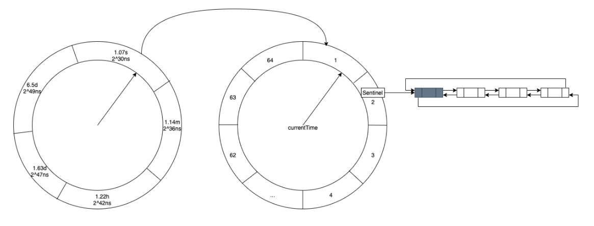
TimerWheel is the implementation of time wheel algorithm. In essence, it is a layered timer, which can add, delete or trigger expired events under the equal sharing time complexity of O(1). The specific implementation of the time wheel is a two-dimensional array, and the specific location of the array is a linked list of nodes to be executed.
The first dimension of the two-dimensional array of time wheels is the specific time interval, which is seconds, minutes, hours, days and 4 days respectively. However, the units are not distinguished strictly according to the time unit, but the time interval is taken as the time interval according to the integer power of 2 closest to the above units. Therefore, the time intervals in the first dimension are 1.07s, 1.14m, 1.22h, 1.63d and 6.5d respectively.
final class TimerWheel<K, V> {
  // Number of bucket s of wheel on each layer of time wheel
  static final int[] BUCKETS = { 64, 64, 32, 4, 1 };
  // Time span of wheel on each floor of time wheel
  static final long[] SPANS = {
      ceilingPowerOfTwo(TimeUnit.SECONDS.toNanos(1)), // 1.07s = 2^30ns = 1,073,741,824 ns
      ceilingPowerOfTwo(TimeUnit.MINUTES.toNanos(1)), // 1.14m = 2^36ns = 68,719,476,736 ns
      ceilingPowerOfTwo(TimeUnit.HOURS.toNanos(1)),   // 1.22h = 2^42ns = 4,398,046,511,104 ns
      ceilingPowerOfTwo(TimeUnit.DAYS.toNanos(1)),    // 1.63d = 2^47ns = 140,737,488,355,328 ns
      BUCKETS[3] * ceilingPowerOfTwo(TimeUnit.DAYS.toNanos(1)), // 6.5d = 2^49ns = 562,949,953,421,312 ns
      BUCKETS[3] * ceilingPowerOfTwo(TimeUnit.DAYS.toNanos(1)), // 6.5d = 2^49ns = 562,949,953,421,312 ns
  };
  // Displacement deviation of wheel on each floor of time wheel
  static final long[] SHIFT = {
      Long.numberOfTrailingZeros(SPANS[0]),		// 30
      Long.numberOfTrailingZeros(SPANS[1]),		// 36
      Long.numberOfTrailingZeros(SPANS[2]),		// 42
      Long.numberOfTrailingZeros(SPANS[3]),		// 47
      Long.numberOfTrailingZeros(SPANS[4]),		// 49
  };

  final BoundedLocalCache<K, V> cache;
  final Node<K, V>[][] wheel;

  long nanos;

  // Initialize wheel, a two-dimensional array
  @SuppressWarnings({"rawtypes", "unchecked"})
  TimerWheel(BoundedLocalCache<K, V> cache) {
    this.cache = requireNonNull(cache);

    // Each element in the wheel is a Node. The first dimension is the number of BUCKETS, that is, 5, which represents the number of layers of the time wheel
    wheel = new Node[BUCKETS.length][1];
    for (int i = 0; i < wheel.length; i++) {
      // The second dimension represents the number of bucket s in each layer of time wheel, which are 64, 64, 32, 4 and 1 respectively
      wheel[i] = new Node[BUCKETS[i]];
      // What is stored in the wheel is the sentinel of the bidirectional linked list (a dummy object used to simplify the boundary problem)
      for (int j = 0; j < wheel[i].length; j++) {
        wheel[i][j] = new Sentinel<>();
      }
    }
  }

  /**
   * Advance the time and expel the expired elements
   */
  public void advance(long currentTimeNanos) {
    long previousTimeNanos = nanos;
    try {
      nanos = currentTimeNanos;

      // If wrapping, temporarily shift the clock for a positive comparison
      if ((previousTimeNanos < 0) && (currentTimeNanos > 0)) {
        previousTimeNanos += Long.MAX_VALUE;
        currentTimeNanos += Long.MAX_VALUE;
      }

      for (int i = 0; i < SHIFT.length; i++) {
        // Unsigned right shift (> > sign propagating, > > > zero fill right shift)
        long previousTicks = (previousTimeNanos >>> SHIFT[i]);
        long currentTicks = (currentTimeNanos >>> SHIFT[i]);
        // If the current time and the previous time fall in the same bucket or lag behind the previous time, it means that there is no need to move forward and end
        if ((currentTicks - previousTicks) <= 0L) {
          break;
        }
        // Handle the elements in the bucket between the previous and the current tick, invalid elements or put the surviving elements into the appropriate bucket
        expire(i, previousTicks, currentTicks);
      }
    } catch (Throwable t) {
      nanos = previousTimeNanos;
      throw t;
    }
  }

  /**
   * Expires entries or reschedules into the proper bucket if still active.
   *
   * @param index the wheel being operated on
   * @param previousTicks the previous number of ticks
   * @param currentTicks the current number of ticks
   */
  void expire(int index, long previousTicks, long currentTicks) {
    Node<K, V>[] timerWheel = wheel[index];
    int mask = timerWheel.length - 1;

    int steps = Math.min(1 + Math.abs((int) (currentTicks - previousTicks)), timerWheel.length);
    int start = (int) (previousTicks & mask);
    int end = start + steps;

    for (int i = start; i < end; i++) {
      Node<K, V> sentinel = timerWheel[i & mask];
      Node<K, V> prev = sentinel.getPreviousInVariableOrder();
      Node<K, V> node = sentinel.getNextInVariableOrder();
      sentinel.setPreviousInVariableOrder(sentinel);
      sentinel.setNextInVariableOrder(sentinel);

      while (node != sentinel) {
        Node<K, V> next = node.getNextInVariableOrder();
        node.setPreviousInVariableOrder(null);
        node.setNextInVariableOrder(null);

        try {
          if (((node.getVariableTime() - nanos) > 0)
              || !cache.evictEntry(node, RemovalCause.EXPIRED, nanos)) {
            schedule(node);
          }
          node = next;
        } catch (Throwable t) {
          node.setPreviousInVariableOrder(sentinel.getPreviousInVariableOrder());
          node.setNextInVariableOrder(next);
          sentinel.getPreviousInVariableOrder().setNextInVariableOrder(node);
          sentinel.setPreviousInVariableOrder(prev);
          throw t;
        }
      }
    }
  }

  /**
   * Schedules a timer event for the node.
   *
   * @param node the entry in the cache
   */
  public void schedule(@NonNull Node<K, V> node) {
    Node<K, V> sentinel = findBucket(node.getVariableTime());
    link(sentinel, node);
  }

  /**
   * Reschedules an active timer event for the node.
   *
   * @param node the entry in the cache
   */
  public void reschedule(@NonNull Node<K, V> node) {
    if (node.getNextInVariableOrder() != null) {
      unlink(node);
      schedule(node);
    }
  }

  /**
   * Removes a timer event for this entry if present.
   *
   * @param node the entry in the cache
   */
  public void deschedule(@NonNull Node<K, V> node) {
    unlink(node);
    node.setNextInVariableOrder(null);
    node.setPreviousInVariableOrder(null);
  }

  /**
   * Determines the bucket that the timer event should be added to.
   *
   * @param time the time when the event fires
   * @return the sentinel at the head of the bucket
   */
  Node<K, V> findBucket(long time) {
    // Difference between event trigger time and current time wheel rotation time
    long duration = time - nanos;
    int length = wheel.length - 1;
    for (int i = 0; i < length; i++) {
      // 1.07s, 1.14m, 1.22h, 1.63d, 6.5d
      // If the time difference is smaller than the span of the next time wheel, it will fall on the current time wheel. For example, if the time difference is 20s, less than 1.14m, it will fall on the first floor wheel[0]
      if (duration < SPANS[i + 1]) {
        // Calculate which bucket should fall in the first layer and map it to one of them through the hash function
        long ticks = (time >>> SHIFT[i]);
        int index = (int) (ticks & (wheel[i].length - 1));
        return wheel[i][index];
      }
    }
    // Put it on the top floor without a suitable position
    return wheel[length][0];
  }

  /** Adds the entry at the tail of the bucket's list. */
  // Double linked list tail interpolation with sentinel node
  void link(Node<K, V> sentinel, Node<K, V> node) {
    node.setPreviousInVariableOrder(sentinel.getPreviousInVariableOrder());
    node.setNextInVariableOrder(sentinel);

    sentinel.getPreviousInVariableOrder().setNextInVariableOrder(node);
    sentinel.setPreviousInVariableOrder(node);
  }

  /** Removes the entry from its bucket, if scheduled. */
  void unlink(Node<K, V> node) {
    Node<K, V> next = node.getNextInVariableOrder();
    if (next != null) {
      Node<K, V> prev = node.getPreviousInVariableOrder();
      next.setPreviousInVariableOrder(prev);
      prev.setNextInVariableOrder(next);
    }
  }

  /** Returns the duration until the next bucket expires, or {@link Long.MAX_VALUE} if none. */
  @SuppressWarnings("IntLongMath")
  public long getExpirationDelay() {
    for (int i = 0; i < SHIFT.length; i++) {
      Node<K, V>[] timerWheel = wheel[i];
      long ticks = (nanos >>> SHIFT[i]);

      long spanMask = SPANS[i] - 1;
      int start = (int) (ticks & spanMask);
      int end = start + timerWheel.length;
      int mask = timerWheel.length - 1;
      for (int j = start; j < end; j++) {
        Node<K, V> sentinel = timerWheel[(j & mask)];
        Node<K, V> next = sentinel.getNextInVariableOrder();
        if (next == sentinel) {
          continue;
        }
        long buckets = (j - start);
        long delay = (buckets << SHIFT[i]) - (nanos & spanMask);
        delay = (delay > 0) ? delay : SPANS[i];

        for (int k = i + 1; k < SHIFT.length; k++) {
          long nextDelay = peekAhead(k);
          delay = Math.min(delay, nextDelay);
        }

        return delay;
      }
    }
    return Long.MAX_VALUE;
  }

}
Overall structure of time wheel
| Layer (wheel) | Scale (bucket) | Time span of each floor (span) | Shift digit | Tick time |
|---|---|---|---|---|
| 1 | 64 | 1.07s = 2^30ns = 1,073,741,824 ns | 30 | 2^30 /64 = 2^24 ns = 16.7ms |
| 2 | 64 | 1.14m = 2^36ns = 68,719,476,736 ns | 36 | 2^36 /64 = 2^30 ns = 1.07s |
| 3 | 32 | 1.22h = 2^42ns = 4,398,046,511,104 ns | 42 | 2^42 /32 = 2^37 ns = 2.29m |
| 4 | 4 | 1.63d = 2^47ns = 140,737,488,355,328 ns | 47 | 2^47 /4 = 2^45 ns = 9.77h |
| 5 | 1 | 6.5d = 2^49ns = 562,949,953,421,312 ns | 49 | 2^49 /1 = 6.5d |
To be continued
summary
TODO