Article catalog
1. Learning objectives
- Understand simple and logarithmic returns
- Calculate the return on investment for different stocks through Pandas and NumPy
- Calculate the return of the portfolio by linear summation
2. Operation explanation
Starting from this task, we will use Python and its related software packages for data analysis in the field of investment.
Any investment should consider two points: possible gains and possible losses. People always want to increase the opportunity to gain and reduce the risk of loss. However, the two are "fish and bear's paw can't have both", and usually high income means high risk.
For example, the interest rate of time deposits in banks is very low, but as long as the banks do not fail, the principal is always guaranteed. In contrast, the futures market means high returns in the short term, but it may also make investors suffer huge principal losses. So how to evaluate the return and risk of an investment in a scientific way and find a relative equilibrium point?
Don't worry, let's look at it step by step.
The first is the definition of the rate of return. There are usually two ways to calculate the rate of return: Simple Rate of Return and Logarithm Rate of Return.

Generally, when comparing different types of investments, from the perspective of dimension, simple rate of return is used in most cases, while logarithmic rate of return can be used to compare different stages of the same investment.
To understand the rate of return, we need to predict the return of investment in the future. Of course, because there are too many factors affecting investment in the real world, it is impossible for us to do everything and make a completely accurate model. Therefore, strictly speaking, the future is unpredictable. All we can do is make a rough guess according to the historical behavior of investment, so as to approximate people's expectations for the future. Here, we evaluate and predict through the historical data of the stock market. Obtain the stock price data of Alibaba, JD and Tencent in the stock market.
import numpy as np
import pandas as pd

# Obtain Alibaba's share price data in January 2021
BABA = pd.read_csv('./BABA.csv', sep='\t', index_col=0)

# Display the first few pieces of data
print('Alibaba's share price in early January 2021', BABA.head())
# Display the last few pieces of data
print('Alibaba's share price at the end of January 2021', BABA.tail())
print()

# Obtain the share price data of JD in January 2021
JD = pd.read_csv('./JD.csv', sep='\t', index_col=0)
# Display the first few pieces of data
print('JD's share price in early January 2021', JD.head())
# Display the last few pieces of data
print('JD's share price at the end of January 2021', JD.tail())
print()

# Obtain Tencent's share price data in January 2021
TC = pd.read_csv('./TC.csv', sep='\t', index_col=0)
# Display the first few pieces of data
print('Tencent's share price in early January 2021', TC.head())
# Display the last few pieces of data
print('Tencent's share price at the end of January 2021', TC.tail())
print()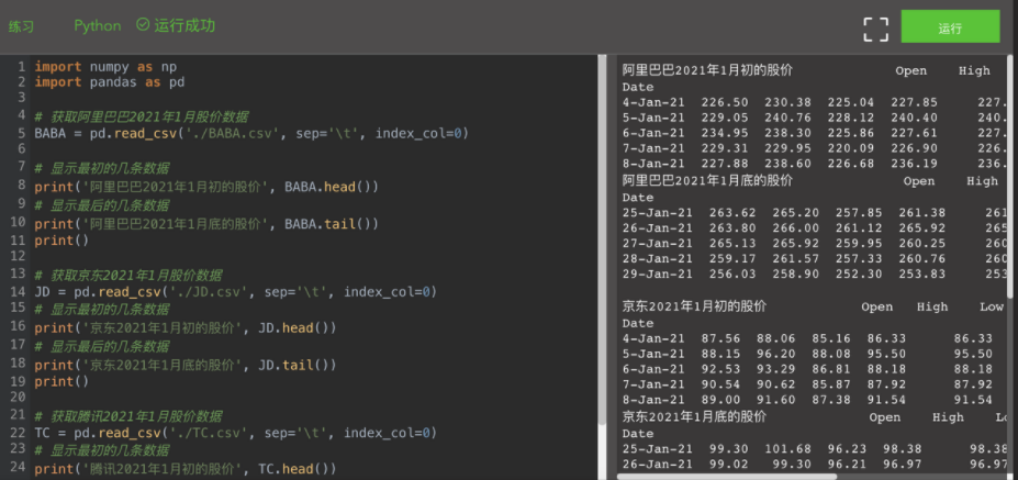
Here we pass three csv file to obtain the share prices of Alibaba (stock code BABA), JD (stock code JD) and Tencent (stock code TCTZF) from January 2021. Pandas read_ The stock data returned by csv () function is stored in the form of pandas dataframe. This data structure is similar to the table in relational database. Rows represent records and lists show fields or attributes. Then we can operate on these dataframes, for example, using the following code to obtain a simple rate of return every day.
# Get Alibaba's simple rate of return
BABA['simple_return'] = round((BABA['Adj Close'] / BABA['Adj Close'].shift(1)) - 1, 4)
print(BABA['simple_return'])
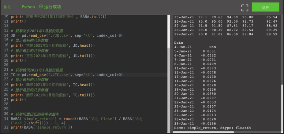
In the above code, BABA ['simple_return'] means that a new one named simple is added to the dataframe of Alibaba stock data_ Return column, whose value is round((BABA ['Adj Close '] / BABA ['Adj Close']. Shift (1)) - 1,4).
The function round () has the same function as the function round () in SQL, and both retain several digits after the decimal point. The focus of simple yield is (BABA ['Adj Close '] / BABA ['Adj Close'. shift(1)) - 1. Here, BABA ['Adj Close '] represents the adjusted closing price of the day, while BABA ['Adj Close'] shift(1) refers to the adjusted closing price of the previous day, and shift(1) refers to the previous day.
Because of this, there is no yield on the first day, because there is no comparison base in front. You will see in the final result of yield calculation that the yield on the first day is NaN. Please practice and calculate the simple yield of JD and Tencent every day.
Next, we use the following code to calculate the daily average simple rate of return and annual average simple rate of return for these days.
# Get Alibaba's daily average simple rate of return
print('Alibaba's daily average simple rate of return', round(BABA['simple_return'].mean() * 100, 4), '%')
# Obtain Alibaba's annual average simple rate of return
print('Alibaba's annual average simple rate of return', round(BABA['simple_return'].mean() * 250 * 100, 4), '%')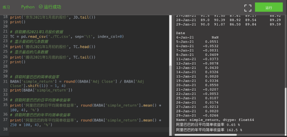
Through BABA ['simple_return'] mean() gets the average value of the simple rate of return, that is, the daily average simple rate of return. Then we assume that there are 250 trading days in a year, then the average annual simple yield in that year is 250 times the previous daily average. In addition, the code converts the decimal to a percentage that retains four digits after the decimal point. Please use a similar method to obtain the daily average and average annual simple rate of return of JD and Tencent.
Similarly, we can calculate logarithmic returns for these stocks. The following code lists Alibaba's daily average logarithmic rate of return and annual average logarithmic rate of return.
# Get Alibaba's daily average logarithmic rate of return
BABA['log_return'] = round(np.log((BABA['Adj Close'] / BABA['Adj Close'].shift(1))), 4)
print('Alibaba's daily average log yield', round(BABA['log_return'].mean() * 100, 4), '%')
# Obtain Alibaba's annual average logarithmic rate of return
print('Alibaba's annual average logarithmic rate of return', round(BABA['log_return'].mean() * 250 * 100, 4), '%')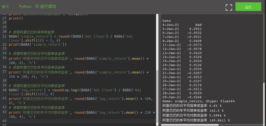
Please use a similar method to obtain the daily average and average annual logarithmic returns of JD and Tencent. The complete code before is listed below for your reference:
import numpy as np
import pandas as pd

# Obtain Alibaba's share price data in January 2021
BABA = pd.read_csv('./BABA.csv', sep='\t', index_col=0)

# Display the first few pieces of data
print('Alibaba's share price in early January 2021', BABA.head())
# Display the last few pieces of data
print('Alibaba's share price at the end of January 2021', BABA.tail())
print()

# Obtain the share price data of JD in January 2021
JD = pd.read_csv('./JD.csv', sep='\t', index_col=0)
# Display the first few pieces of data
print('JD's share price in early January 2021', JD.head())
# Display the last few pieces of data
print('JD's share price at the end of January 2021', JD.tail())
print()

# Obtain Tencent's share price data in January 2021
TC = pd.read_csv('./TC.csv', sep='\t', index_col=0)
# Display the first few pieces of data
print('Tencent's share price in early January 2021', TC.head())
# Display the last few pieces of data
print('Tencent's share price at the end of January 2021', TC.tail())
print()


# Get Alibaba's simple rate of return
BABA['simple_return'] = round((BABA['Adj Close'] / BABA['Adj Close'].shift(1)) - 1, 4)
print(BABA['simple_return'])

# Get Alibaba's daily average simple rate of return
print('Alibaba's daily average simple rate of return', round(BABA['simple_return'].mean() * 100, 4), '%')
# Obtain Alibaba's annual average simple rate of return
print('Alibaba's annual average simple rate of return', round(BABA['simple_return'].mean() * 250 * 100, 4), '%')


# Get Alibaba's daily average logarithmic rate of return
BABA['log_return'] = round(np.log((BABA['Adj Close'] / BABA['Adj Close'].shift(1))), 4)
print('Alibaba's daily average log yield', round(BABA['log_return'].mean() * 100, 4), '%')
# Obtain Alibaba's annual average logarithmic rate of return
print('Alibaba's annual average logarithmic rate of return', round(BABA['log_return'].mean() * 250 * 100, 4), '%')
Many times, our investment does not rely on a single type, but consists of a variety of portfolios, such as savings, funds, stocks, real estate and so on. Even if you only invest in one kind, such as stocks, you can own stocks of different companies. At this time, we need to calculate the comprehensive rate of return of the portfolio. Assuming that 30% of the funds you invest in stocks are used to buy Alibaba's stocks, 35% are used to buy JD's stocks, and the last 35% are used to buy Tencent's stocks, the comprehensive return on investment is

This linear addition method is the same as that we used to calculate the comprehensive similarity. The following code is the specific implementation:
import numpy as np
import pandas as pd

# Use multiple stock codes to build a new dataframe
BABA = pd.read_csv('./BABA.csv', sep='\t', index_col=0)
JD = pd.read_csv('./JD.csv', sep='\t', index_col=0)
TC = pd.read_csv('./TC.csv', sep='\t', index_col=0)

stock_data = pd.DataFrame()
stock_data['BABA'] = BABA['Adj Close']
stock_data['JD'] = JD['Adj Close']
stock_data['TCTZF'] = TC['Adj Close']

# Get the daily simple yield of all stocks
returns = stock_data / stock_data.shift(1) - 1
print(returns)

# Set the capital proportion of each stock
weights = np.array([0.3, 0.35, 0.35])
# Through linear addition, the comprehensive simple rate of return is calculated
combined_return = np.dot(returns, weights)
print(combined_return)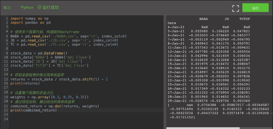
The above code creates a new one named stock_ The dataframe of data, in which each column corresponds to the one-day closing price of a stock. Such a stock_data is also a matrix. You can use stock directly_ data / stock_data. Shift (1) - 1 completes the simple one-day yield calculation for each column (that is, each stock). The resulting returns variable is also a matrix structure, so we use NP Array and NP Dot realizes the point multiplication of stock return matrix returns and weight vector weights, and finally obtains the daily comprehensive simple return, which is the weighted average of each stock.
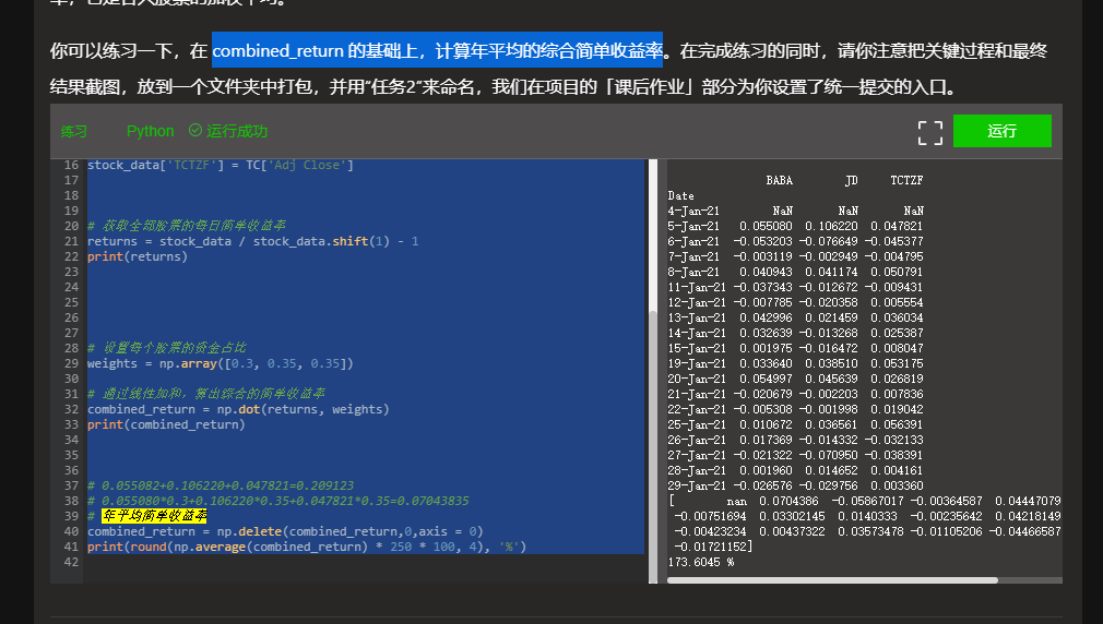
You can practice in combined_return to calculate the annual average comprehensive simple rate of return. While completing the exercise, please pay attention to put the screenshots of the key process and final results into a folder, package them and name them with "task 2". We have set a unified submission entry for you in the "homework" part of the project.
3. Job results
# -*- coding: utf-8 -*-
# @Software: PyCharm
# @File : Task2.py
# @Author : Benjamin
# @Time : 2021/9/10 10:10


import numpy as np
import pandas as pd


# Use multiple stock codes to build a new dataframe
BABA = pd.read_csv('../baba.csv', sep='\t', index_col=0)
JD = pd.read_csv('../jd.csv', sep='\t', index_col=0)
TC = pd.read_csv('../tc.csv', sep='\t', index_col=0)

stock_data = pd.DataFrame()
stock_data['BABA'] = BABA['Adj Close']
stock_data['JD'] = JD['Adj Close']
stock_data['TCTZF'] = TC['Adj Close']


# Get the daily simple yield of all stocks
returns = stock_data / stock_data.shift(1) - 1
print(returns)


# Set the capital proportion of each stock
weights = np.array([0.3, 0.35, 0.35])

# Through linear addition, the comprehensive simple rate of return is calculated
combined_return = np.dot(returns, weights)
print(combined_return)


# 0.055082+0.106220+0.047821=0.209123
# 0.055080*0.3+0.106220*0.35+0.047821*0.35=0.07043835
# Annual average simple rate of return
# Through BABA ['simple_return'] mean() gets the average value of the simple rate of return, that is, the daily average simple rate of return. Then we assume that there are 250 trading days in a year, then the average annual simple yield in that year is 250 times the previous daily average. In addition, the code converts the decimal to a percentage that retains four digits after the decimal point. Please use a similar method to obtain the daily average and average annual simple rate of return of JD and Tencent.
combined_return = np.delete(combined_return,0,axis = 0)
print(round(np.average(combined_return) * 250 * 100, 4), '%')
If you think the article is good, then point a praise and a collection.
WeChat official account, and tweets later.