The space here may be too long. Carry out the water alone. The tutorial video is only eight minutes long. I just looked at my ideas, and then I wrote it for two hours. I kept fixing mistakes, and finally came up with a result similar to the result in the video.
Problem description
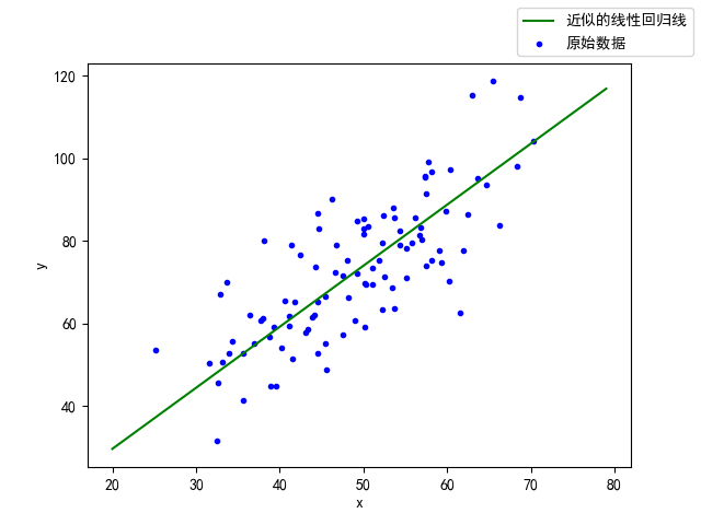
According to the first-order equation of last class: y=1.477x+0.089
On the basis of this equation, add noise to generate 100 groups of data, and then use the method of linear regression to approximate the parameters of the equation. w and b in y=wx+b

Overall code
No more nonsense, just code first
#!usr/bin/env python
# -*- coding:utf-8 -*-
"""
@author: Temmie
@file: test.py
@time: 2021/05/10
@desc:
"""
import pandas as pd
from matplotlib import pyplot
import numpy
#Prevent Chinese garbled code
from matplotlib import font_manager
font_manager.FontProperties(fname='C:\Windows\Fonts\AdobeSongStd-Light.otf')
pyplot.rcParams['font.sans-serif']=['SimHei'] #Used to display Chinese labels normally
pyplot.rcParams['axes.unicode_minus']=False #Used to display negative signs normally
def loss_cal(w,b,x,y):#Loss function calculation
loss_value=0
for i in range(len(x)):
loss_value +=(w*x[i]+b-y[i])**2
return loss_value/(len(x))
def change_wb(w,b,x,y,learn_rate):#Modification of w and b
gra_w_t=0
gra_b_t=0a
for i in range(len(x)):
gra_w_t +=(2*(w*x[i]+b-y[i])*x[i])/(len(x))
gra_b_t +=(2*(w*x[i]+b-y[i]))/(len(x))
w_now=w-learn_rate*gra_w_t
b_now=b-learn_rate*gra_b_t
return w_now,b_now
def the_res(x,y,sx,sy,loss):#Draw an image to display the results
pyplot.scatter(x,y,color='blue',marker='.',label='raw data')
pyplot.plot(sx,sy,color='green',label='Approximate linear regression line')
pyplot.figlegend()
pyplot.xlabel('x', loc='center')
pyplot.ylabel('y', loc='center')
pyplot.show()
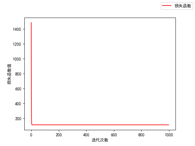
pyplot.plot(loss,color='red',label='loss function ')
pyplot.figlegend()
pyplot.xlabel('Number of iterations', loc='center')
pyplot.ylabel('Loss function value', loc='center')
pyplot.show()
#read in data
df = pd.read_csv('D:\learning_folder\data.csv')
#Separate different data
x=df.loc[:,'x'];print(x)
y=df.loc[:,'y'];print(y)
#Set the initial W and b initialization loss function value loss_v number of iterations w_num and learning rate learn_rate
w=0;b=0;loss_v=[];w_num=1000;learn_rate=0.0001
for i in range(1,w_num,1):
#Calculate loss function
loss_v.append(loss_cal(w,b,x,y))
#Iterative changes w and b
w,b=change_wb(w,b,x,y,learn_rate)
print('w:',w,'\t','b:',b,'\t','final_loss:',loss_v[-1])
#Draw results
sx=numpy.array(list(range(20,80,1)),dtype='float')
sy=w*sx+b
the_res(x,y,sx,sy,loss_v[1:])
Code parsing
Import module
import pandas as pd
from matplotlib import pyplot
import numpy
from matplotlib import font_manager
The first pandas is used to read data files (. csv files) and process the data;
The second pyplot is used for drawing;
The third numpy is also data processing;
The fourth is to prevent Chinese garbled code;
Prevent Chinese garbled code
Fixed content
from matplotlib import font_manager
font_manager.FontProperties(fname='C:\Windows\Fonts\AdobeSongStd-Light.otf')
pyplot.rcParams['font.sans-serif']=['SimHei'] #Used to display Chinese labels normally
pyplot.rcParams['axes.unicode_minus']=False #Used to display negative signs normally
Initialization content
Here, we need to give the initial w and b for iterative calculation, iterative algebra, learning rate, and initialize some empty lists to facilitate the storage of the contents we want to query in the iterative process, such as the change of the value of the loss function.
#Set the initial W and b initialization loss function value loss_v number of iterations w_num and learning rate learn_rate
w=0;b=0;loss_v=[];w_num=1000;learn_rate=0.0001
Cyclic iteration
for i in range(1,w_num,1):
    #Calculate loss function
    loss_v.append(loss_cal(w,b,x,y))
    #Iterative changes w and b
    w,b=change_wb(w,b,x,y,learn_rate)
Don't panic, the loss in here_ Cal and change_wb is a function written by ourselves
Function loss_cal
This is a function for calculating the loss function
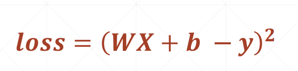
Here's a point to explain: in order to prevent the value of gradient decline from changing frequently, we can use the method of calculating the average value in blocks to prevent the parameters from shaking sharply. Therefore, we calculate the instantaneous function value against 100 groups of data, take the average, and then change the parameters w and b
def loss_cal(w,b,x,y):#Loss function calculation
    loss_value=0
    for i in range(len(x)):
        loss_value +=(w*x[i]+b-y[i])**2
    return loss_value/(len(x))
Function change_wb(w,b,x,y,learn_rate)
This is a function of using gradient descent to update w and b
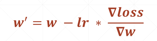
Note that when calculating the gradient of W and b, the derivative is w and b respectively, and the others should be treated as constants
def change_wb(w,b,x,y,learn_rate):#Modification of w and b
    gra_w_t=0
    gra_b_t=0a
    for i in range(len(x)):
        gra_w_t +=(2*(w*x[i]+b-y[i])*x[i])/(len(x))
        gra_b_t +=(2*(w*x[i]+b-y[i]))/(len(x))
    w_now=w-learn_rate*gra_w_t
    b_now=b-learn_rate*gra_b_t
    return w_now,b_now
Display important parameters at the end of iteration
print('w:',w,'\t','b:',b,'\t','final_loss:',loss_v[-1])
Draw the_res(x,y,sx,sy,loss)
This part can refer to the plot part I wrote. If necessary, go to the python column detailed list query
def the_res(x,y,sx,sy,loss):#Draw an image to display the results
    pyplot.scatter(x,y,color='blue',marker='.',label='raw data')
    pyplot.plot(sx,sy,color='green',label='Approximate linear regression line')
    pyplot.figlegend()
    pyplot.xlabel('x', loc='center')
    pyplot.ylabel('y', loc='center')
    pyplot.show()
    pyplot.plot(loss,color='red',label='loss function ')
    pyplot.figlegend()
    pyplot.xlabel('Number of iterations', loc='center')
    pyplot.ylabel('Loss function value', loc='center')
    pyplot.show()
Originally, the y-axis can be used for non-linear drawing, but it was developed by developers and advanced users. In the future, we can understand and supplement the drawing with better effect. In fact, the value of the loss function is not a straight line