1 Introduction to causalnex

1.1 installation

pip install causalnex

github:https://github.com/quantumblacklabs/causalnex
Document link: https://causalnex.readthedocs.io/en/latest/02_getting_started/02_install.html

CausalNex is a Python library that uses Bayesian networks to combine machine learning and domain expertise for causal reasoning.
You can use CausalNex to reveal structural relationships in data, understand complex distributions, and observe the effects of potential interventions.
The CausalNex library has the following features:

• Adopt the most advanced structural learning method, DAG with no teachers, to understand the conditional dependence between variables
• Allow domain knowledge to extend model relationships
• A prediction model based on structural relationship is established
• Understanding probability model
• Evaluate model quality with standard statistical inspection
• Visualization simplifies the understanding of causality
• The impact of interventions was analyzed using calculus

Compared with the traditional machine learning methods based on pattern recognition and correlation analysis, Bayesian network is more intuitive to describe causality.
If domain expertise can be easily coded or added to the graph model, causality will be more accurate.
Graphical models can then be used to assess the impact of changes on potential characteristics, i.e. counterfactual analysis, and to determine the correct intervention.
According to experience, data scientists usually have to use at least 3-4 different open source libraries to reach the last step of finding the right intervention. CausalNex aims to simplify the end-to-end process of causality and counterfactual analysis.

2 model used

2.1 structural equation model of notears

reference resources: DAG_GNN: a DAG structure learning architecture based on VAE

The open source library model refers to NOTEARS model: DAGs with NO TEARS: Continuous Optimization for Structure Learning

Several highlights in the paper:

• In this paper, the acyclic structure constraint of DAG learning is improved from the traditional combination constraint (discrete, acyclic structure increases in geometric multiples) to a smooth continuous constraint( h ( w ) h(w) h(w) )

F(W) is the score function, and DAG_GNN is another upgrade model, which will be used in this h ( w ) h(w) h(w) upgrade;

• h ( w ) h(w) After h(w), X is modeled by the defined structural equation model (SEM), which focuses on finding a SEM that can minimize the loss of least squares (LS).

3 modeling case: NOTEARS structural equation model

3.1 data loading

Case source: Structure-Learning

import pandas as pd

data = pd.read_csv('student-por.csv', delimiter=';')
data.head(5)

# Data processing
drop_col = ['school','sex','age','Mjob', 'Fjob','reason','guardian']
data = data.drop(columns=drop_col)
data.head(5)

import numpy as np

struct_data = data.copy()
non_numeric_columns = list(struct_data.select_dtypes(exclude=[np.number]).columns)
# Data text - > numeric
from sklearn.preprocessing import LabelEncoder
le = LabelEncoder()
for col in non_numeric_columns:
    struct_data[col] = le.fit_transform(struct_data[col])

struct_data.head(5)

After loading the data and performing some numerical operations on the data, the next step is modeling:

from causalnex.structure.notears import from_pandas
sm = from_pandas(struct_data)

It can be seen here that each variable is interconnected because there is no expert assignment and no filtering edge operation, so it is displayed;
Alternatively, you can use remove_edges_below_threshold to set some thresholds for deletion:

sm.remove_edges_below_threshold(0.8)
viz = plot_structure(
    sm,
    graph_attributes={"scale": "0.5"},
    all_node_attributes=NODE_STYLE.WEAK,
    all_edge_attributes=EDGE_STYLE.WEAK,
)
Image(viz.draw(format='png'))

If the edge coefficient threshold is less than 0.8 is deleted, the current figure will appear:

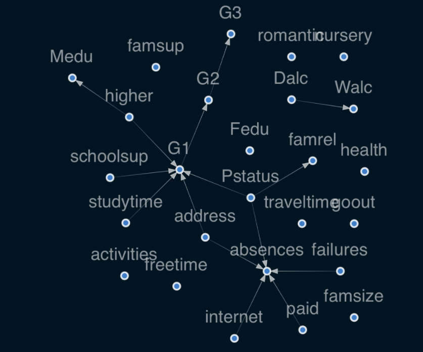
Interpretation of results:

• Family status P s t a t u s Pstatus Pstatus affects family relations f a m r e l famrel famrel - if parents are separated, the quality of family relations may deteriorate.
• network i n t e r n e t internet internet affects absenteeism a b s e n c e s absences absences - having an Internet at home may cause students to skip classes.
• Long learning time s t u d y t i m e studytime studytime on students' grades G 1 G1 G1 has a positive impact.

3.2 operations required for modeling & error pointing

3.2.1 error pointing solution 1: add constraints

Of course, there may also be a wrong direction:
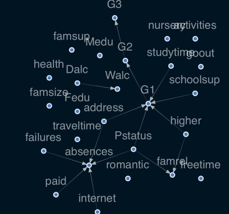
Children's Higher Education h i g h e r higher higher will affect M e d u Medu Medu (mother's education) - this relationship is meaningless because students who want to pursue higher education will not affect their mother's education.
For this wrong direction, some constraints can be added during modeling:

sm = from_pandas(struct_data, tabu_edges=[("higher", "Medu")], w_threshold=0.8)
viz = plot_structure(
    sm,
    graph_attributes={"scale": "0.5"},
    all_node_attributes=NODE_STYLE.WEAK,
    all_edge_attributes=EDGE_STYLE.WEAK,
)
Image(viz.draw(format='png'))

3.2.2 error pointing solution 2: direct fine tuning results

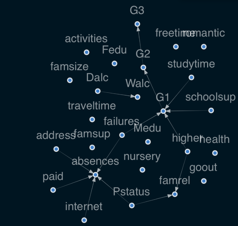
Add / delete edge

sm.add_edge("failures", "G1")
sm.remove_edge("Pstatus", "G1")
sm.remove_edge("address", "G1")

3.3 retrieving the largest subgraph

We can see that there are two independent subgraphs in the visual diagram: dalc - > WALC and another large subgraph.
We can easily retrieve the largest subgraph by calling the StructureModel function get_largest_subgraph().

sm = sm.get_largest_subgraph()
viz = plot_structure(
    sm,
    graph_attributes={"scale": "0.5"},
    all_node_attributes=NODE_STYLE.WEAK,
    all_edge_attributes=EDGE_STYLE.WEAK,
)
Image(viz.draw(format='png'))

3.4 export structure

To export nx#u pydot using networkx:

import networkx as nx

nx.drawing.nx_pydot.write_dot(sm, 'graph.dot')

3.5 fitting conditional distribution of Bayesian network: data discretization

When the edge structure information is confirmed, Bayesian network can be used to fit different characteristic conditional probability distributions.
Bayesian networks in CausalNex only support discrete distribution. Any continuous features, or features with a large number of categories, should be discretized before fitting Bayesian networks. Models containing variables with many possible values are usually not suitable and show poor performance.
For example, consider P(G2 | G1), where G1 and G2 have possible values of 0 to 20. Therefore, the discrete conditional probability distribution is 21 × 21 (441) possible combinations are specified - most of which we will be unlikely to observe.
CausalNex provides some auxiliary methods to simplify discretization. Let's start by reducing the number of categories in some classification features by combining similar values. We will classify digital features through discretization, and then give meaningful labels to buckets.

from causalnex.network import BayesianNetwork
bn = BayesianNetwork(sm)

For example, in the learning time function, we put more than 2 hours (2 means 2 to 5 hours here, see https://archive.ics.uci.edu/ml/datasets/Student +The learning time of performance) is divided into long learning time and the rest into short learning time.

discretised_data = data.copy()

data_vals = {col: data[col].unique() for col in data.columns}

failures_map = {v: 'no-failure' if v == [0]
                else 'have-failure' for v in data_vals['failures']}
studytime_map = {v: 'short-studytime' if v in [1,2]
                 else 'long-studytime' for v in data_vals['studytime']}

discretised_data["failures"] = discretised_data["failures"].map(failures_map)
discretised_data["studytime"] = discretised_data["studytime"].map(studytime_map)

Discretizing digital features
In order to make digital features classified, they must be discretized first.
CausalNex provides an auxiliary class causalnex.discretiser.Discretiser.
Supports a variety of discretization methods.
For our data, a fixed method will be applied to provide static values that define the bucket boundary.
For example, absenteeism will be divided into several parts < 1, 1-9, > = 10.
Each bucket will be marked as a zero based integer.

from causalnex.discretiser import Discretiser

discretised_data["absences"] = Discretiser(method="fixed",
                          numeric_split_points=[1, 10]).transform(discretised_data["absences"].values)
discretised_data["G1"] = Discretiser(method="fixed",
                          numeric_split_points=[10]).transform(discretised_data["G1"].values)
discretised_data["G2"] = Discretiser(method="fixed",
                          numeric_split_points=[10]).transform(discretised_data["G2"].values)
discretised_data["G3"] = Discretiser(method="fixed",
                          numeric_split_points=[10]).transform(discretised_data["G3"].values)

Create labels for numeric properties
To make discrete categories more readable, we can map category labels to something more meaningful, just like mapping category eigenvalues.

absences_map = {0: "No-absence", 1: "Low-absence", 2: "High-absence"}

G1_map = {0: "Fail", 1: "Pass"}
G2_map = {0: "Fail", 1: "Pass"}
G3_map = {0: "Fail", 1: "Pass"}

discretised_data["absences"] = discretised_data["absences"].map(absences_map)
discretised_data["G1"] = discretised_data["G1"].map(G1_map)
discretised_data["G2"] = discretised_data["G2"].map(G2_map)
discretised_data["G3"] = discretised_data["G3"].map(G3_map)

3.6 BN model training

Split the data, training set and test set:

# Split 90% train and 10% test
from sklearn.model_selection import train_test_split

train, test = train_test_split(discretised_data, train_size=0.9, test_size=0.1, random_state=7)

Using the previously learned structural model and discrete data, we can now fit the probability distribution of Bayesian network.
The first step is to specify all states that each node can take. This can be done by data or providing a node value dictionary.
We use the complete data set here to avoid the situation that the state in the test set does not exist in the training set.
For real applications, you might need to provide these states using the dictionary method.

# Model initialization
bn = bn.fit_node_states(discretised_data)
# Fitting conditional probability distribution
bn = bn.fit_cpds(train, method="BayesianEstimator", bayes_prior="K2")

View the conditional probability distributions (CPDS) dictionary of BN model:

bn.cpds["G1"]

3.7 forecast given input data

The prediction method of Bayesian network enables us to use the learned Bayesian network to predict the data.
For example, we want to predict whether a student has passed the exam based on the input data.
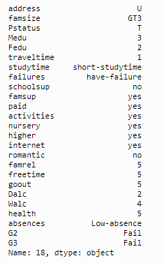
Suppose we have an incoming student data, which is as follows:

discretised_data.loc[18, discretised_data.columns != 'G1']

predictions = bn.predict(discretised_data, "G1")
print(f"The prediction is '{predictions.loc[18, 'G1_prediction']}'")

Student No. 18, the study time here is expressed as short-study time, which feels impossible.

The prediction is 'Fail'

The prediction result here is also fail, which is reasonable.

3.8 model evaluation: classification report + ROC/AUC

3.8.1 Classification Report

from causalnex.evaluation import classification_report

classification_report(bn, test, "G1")

Output results:

{'G1_Fail': {'precision': 0.7777777777777778,
  'recall': 0.5833333333333334,
  'f1-score': 0.6666666666666666,
  'support': 12},
 'G1_Pass': {'precision': 0.9107142857142857,
  'recall': 0.9622641509433962,
  'f1-score': 0.9357798165137615,
  'support': 53},
 'accuracy': 0.8923076923076924,
 'macro avg': {'precision': 0.8442460317460317,
  'recall': 0.7727987421383649,
  'f1-score': 0.8012232415902141,
  'support': 65},
 'weighted avg': {'precision': 0.8861721611721611,
  'recall': 0.8923076923076924,
  'f1-score': 0.8860973888496825,
  'support': 65}}

3.8.2 ROC/AUC

from causalnex.evaluation import roc_auc
roc, auc = roc_auc(bn, test, "G1")
print(auc)

3.9 Querying Marginals

3.9.1 basic query: baseline margins

If you want to query the probability values of some nodes, the previous model cannot be queried. Now you need to rebuild a query engine:

bn = bn.fit_cpds(discretised_data, method="BayesianEstimator", bayes_prior="K2")
from causalnex.inference import InferenceEngine

ie = InferenceEngine(bn)
marginals = ie.query()
marginals["G1"]
>>> {'Fail': 0.25260687281677224, 'Pass': 0.7473931271832277}

Get the conditional probability of each node. Here you can see the node G1. 0.252 is the number of fial and 0.747 is pass
The overall figures can be obtained for checking calculation, which is consistent

import numpy as np

labels, counts = np.unique(discretised_data["G1"], return_counts=True)
list(zip(labels, counts))

3.9.2 query criteria

We can also query the marginal likelihood of states in the network given some observations.
These observations can be made anywhere in the network, and their impact will spread through the nodes of interest.
Let's look at the possibility of G1 according to the study time.

marginals_short = ie.query({"studytime": "short-studytime"})
marginals_long = ie.query({"studytime": "long-studytime"})
print("Marginal G1 | Short Studtyime", marginals_short["G1"])
print("Marginal G1 | Long Studytime", marginals_long["G1"])

Output is:

Marginal G1 | Short Studtyime {'Fail': 0.2776556433482524, 'Pass': 0.7223443566517477}
Marginal G1 | Long Studytime {'Fail': 0.15504850337837614, 'Pass': 0.8449514966216239}

It can be seen here that 0.722 of G1 is passed if there is Short Studtyime status;
With Long Studytime status, 0.844 of G1 is passed

So relatively speaking, Long Studytime is easier to pass than short studytime.

3.10 [final / core link] Do Calculus - under confounding factor

We can apply intervention to any node in the data and update its distribution using the do operator. This can be thought of as asking our model "what if it's different".
For example, we can ask, what happens if 100% of students want to continue higher education:

print("marginal G1", ie.query()["G1"])
ie.do_intervention("higher",
                   {'yes': 1.0,
                    'no': 0.0})
print("updated marginal G1", ie.query()["G1"])

Conclusion:

marginal G1 {'Fail': 0.25260687281677224, 'Pass': 0.7473931271832277}
updated marginal G1 {'Fail': , 'Pass': 0.79?????}

It can be seen here that if 90% of people are willing to continue to receive higher education, the G1 score is 0.74;
If it rises to 100% willingness to accept, the average score of G1 will increase to 0.79

4 scikit learn integration interface

DAGRegressor / DAGClassifier is the regression / classification function of scikit learn

It looks more convenient to use here.

4.1 linear regression: Linear DAGRegressor

from sklearn.datasets import load_diabetes
import torch
torch.manual_seed(42)
data = load_diabetes()
X, y = data.data, data.target
names = data["feature_names"]

from sklearn.preprocessing import StandardScaler
ss = StandardScaler()
X = ss.fit_transform(X)
y = (y - y.mean()) / y.std()

from causalnex.structure import DAGRegressor
reg = DAGRegressor(
    alpha=0.1,
    beta=0.9,
    hidden_layer_units=None,
    dependent_target=True,
    enforce_dag=True,
)

from sklearn.model_selection import cross_val_score
from sklearn.model_selection import KFold
scores = cross_val_score(reg, X, y, cv=KFold(shuffle=True, random_state=42))
print(f'MEAN R2: {np.mean(scores).mean():.3f}')

X = pd.DataFrame(X, columns=names)
y = pd.Series(y, name="DPROG")
reg.fit(X, y)
print(pd.Series(reg.coef_, index=names))
reg.plot_dag(enforce_dag=True)

Simultaneous output:

MEAN R2: 0.478
age    0.000000
sex    0.000000
bmi    0.304172
bp     0.000000
s1     0.000000
s2     0.000000
s3     0.000000
s4     0.000000
s5     0.277010
s6     0.000000
dtype: float64

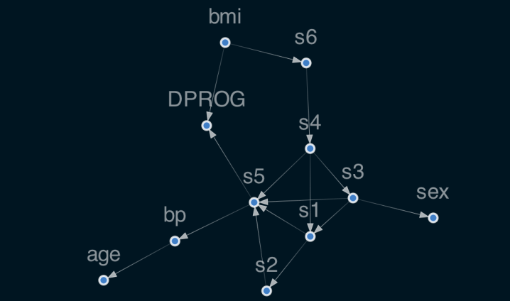
Here are some special model parameters,

• dependent_target: whether X - > y and Y - > x are the same. If it is true, it can point backwards. The default is true
• enforce_dag, whether to delete some edges when displaying the visualization diagram, but it will not be deleted when actually running the model. The default is on

4.2 nonlinear regression

In the process of data processing, it is important to standardize the data

from sklearn.datasets import load_diabetes
import torch
torch.manual_seed(42)
data = load_diabetes()
X, y = data.data, data.target
names = data["feature_names"]

from causalnex.structure import DAGRegressor
reg = DAGRegressor(
    threshold=0.0,
    alpha=0.0001,
    beta=0.2,
    hidden_layer_units=[2],
    standardize=True,
    enforce_dag=True,
)

from sklearn.model_selection import cross_val_score
from sklearn.model_selection import KFold
scores = cross_val_score(reg, X, y, cv=KFold(shuffle=True, random_state=42))
print(f'MEAN R2: {np.mean(scores).mean():.3f}')

X = pd.DataFrame(X, columns=names)
y = pd.Series(y, name="DPROG")
reg.fit(X, y)
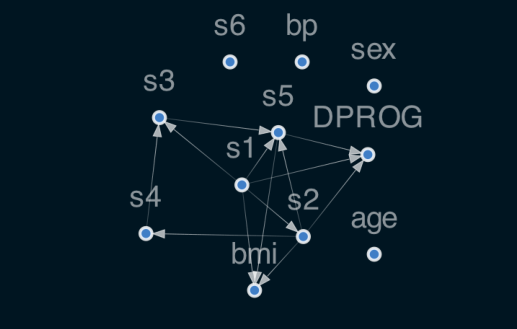
reg.plot_dag(enforce_dag=True)

The nonlinear layer contains s-type nonlinearity, which will be saturated by unscaled data.
In addition, the non scaled data means that the regularization parameters will not have the same impact on the weight of each feature.
Where, standardize = True, which means standardizing X/Y.

It also performs the inverse transformation of y on predict, similar to sklearn transformatedtargetregressor.

4.3 classification model: DAGClassifier

from sklearn.datasets import load_breast_cancer
data = load_breast_cancer()
X, y = data.data, data.target
names = data["feature_names"]

from causalnex.structure import DAGClassifier
clf = DAGClassifier(
    alpha=0.1,
    beta=0.9,
    hidden_layer_units=[5],
    fit_intercept=True,
    standardize=True
)

from sklearn.model_selection import cross_val_score
from sklearn.model_selection import KFold
scores = cross_val_score(clf, X, y, cv=KFold(shuffle=True, random_state=42))
print(f'MEAN Score: {np.mean(scores).mean():.3f}')

X = pd.DataFrame(X, columns=names)
y = pd.Series(y, name="NOT CANCER")
clf.fit(X, y)
for i in range(clf.coef_.shape[0]):
    print(f"MEAN EFFECT DIRECTIONAL CLASS {i}:")
    print(pd.Series(clf.coef_[i, :], index=names).sort_values(ascending=False))
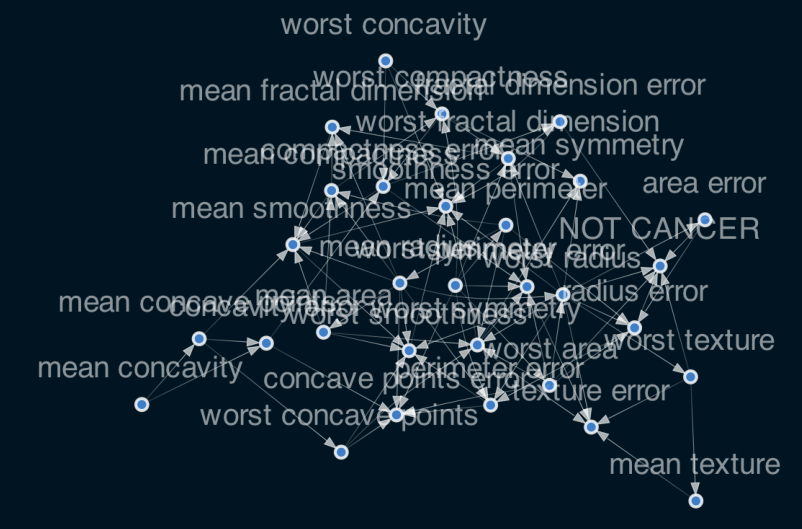
clf.plot_dag(True)

Output:

MEAN Score: 0.975
MEAN EFFECT DIRECTIONAL CLASS 0:
fractal dimension error    0.435006
texture error              0.253090
mean compactness           0.225626
symmetry error             0.112259
compactness error          0.094851
worst compactness          0.087924
mean fractal dimension     0.034403
concavity error            0.030805
mean texture               0.024233
mean symmetry             -0.000012
mean perimeter            -0.000603
mean area                 -0.003670
mean radius               -0.005750
mean smoothness           -0.007812
perimeter error           -0.021268
concave points error      -0.088604
smoothness error          -0.173150
worst smoothness          -0.174532
worst fractal dimension   -0.193018
worst perimeter           -0.241930
worst concavity           -0.251617
worst symmetry            -0.253782
worst concave points      -0.255410
mean concavity            -0.317477
mean concave points       -0.322275
worst area                -0.427581
worst radius              -0.448448
radius error              -0.489342
area error                -0.518434
worst texture             -0.614594
dtype: float64