The theoretical part of this content comes from Chapter 2 "Digital Fourier Transforms" of Numerical Simulation Of Optical Wave Propagation With Example In Matlab

When carrying out discrete Fourier transform for band limited function, attention should be paid to the length of sampling interval and calculation interval.

(1) To calculate the DFT of sinc function.

Define signal function as:

Then the Fourier transform result of numerical analysis is:

 

Then the maximum frequency of the above formula is.

According to Nyquist sampling theorem, the sampling frequency of signal function should be, the sampling interval shall be

Since the book did not give a specific program, I coded it myself.

close all;clear all;clc;
% function values to be used in DFT
a = 1;                       % 
fc = a/2;                    % cutoff frequency of sinc(ax) function
fs = 2*fc;                   % Nyquist Sampling Theorem  - Spatial domain sampling frequency
b = 0.85;                    % Parameters for adjusting sampling interval
delta= b*1/fs;               % Spatial domain sampling interval
N = 100;                     % Sampling points
x = (-N/2:N/2-1)*delta;      % Spatial domain discrete sampling interval
f = (-N/2:N/2-1)/(N*delta);  % Discrete sampling interval in spatial frequency domain
g_samp = sinc(a*x);          %sinc function
g_dft = ft(g_samp, delta);   %DFT

% analytic function % its continuous FT
M = 1024;
x_cont = linspace(x(1),x(end),M);
f_cont = linspace(f(1),f(end),M);
g_cont = sinc(a*x_cont);
g_ft_cont = 1/a*rect(f_cont,a);

% plot
figure('name','Signal function Amplitude'),
plot(x,g_samp,'*',x_cont,g_cont,'-','linewidth',1.2)
legend('Numeric','Analytic');
xlabel('x[m]'); ylabel('g(x)');
grid on

figure('name','DTF Amplitude'),
plot(f,g_dft.*conj(g_dft),'',f_cont,g_ft_cont.*conj(g_ft_cont),'--','linewidth',1.2)
xlim([-1,1]); ylim([-0.1,1.1]);
legend('Numeric','Analytic');
xlabel('f_{x}[m^{-1}]'); ylabel('G(f_{x})');
grid on

Among them, DFT function and rect function are provided by books, as follows:

function G = ft(g, delta)
% function G = ft(g, delta)
G = fftshift(fft(fftshift(g)))*delta;

function y = rect(x,D)
% matlab code for evaluating the rect function
    if nargin == 1
        D = 1;
    end
    x = abs(x);
    y = double(x<D/2);
    y(x == D/2) = 0.5;
    

According to different parameters, there will be some differences in the shape of the drawn image:

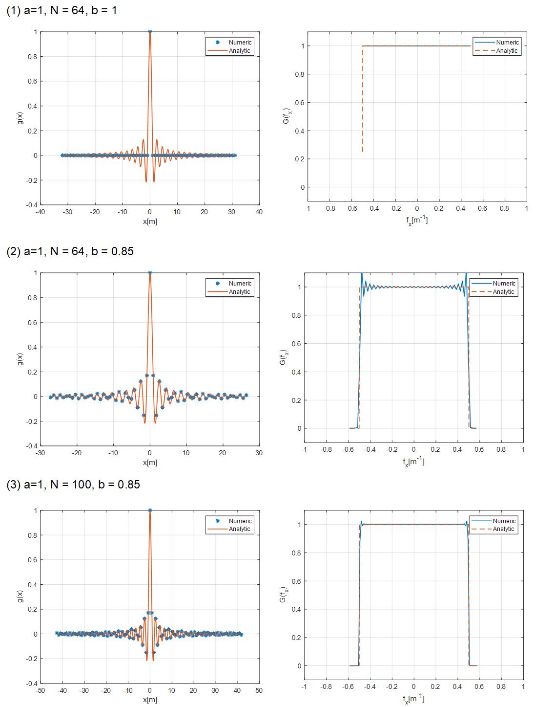
At first, when b = 1, discrete sampling is carried out according to the sampling interval and sampling frequency of Nyquist sampling theorem "standard configuration" and DFT is calculated. However, it is found that the function generated by DFT is a little reluctant; Therefore, the sampling interval in the spatial domain is reduced again, and the parameter b = 0.85 is given. In this way, the sinc function will be sampled more in the spatial domain, and the appearance of the function after DFT is closer to the theoretical analysis function itself.

When changing the number of sampling points n, the more the number of N, the function after DFT can be seen, and its ripple is less at high frequency.

(2) Calculate the DFT of Gaussian function with quadratic phase (degenerate to conventional Gaussian function when b is 0):

spatial domain signal function : 

The corresponding spatial frequency domain analytical ft function is:,

Then its strength isThe cut-off frequency at can be calculated as:

The matlab program has also roughly coded:

close all;clear all;clc;
% function values to be used in DFT
a = 0.25;                    % Amplitude modulation factor
b = 0.57;                    % Quadratic phase modulation factor
% p = 1/exp(2);                % 1/e^2
p = 0.001;                    % 
fc = sqrt(-((a^2+b^4/a^2)/pi)*log(p)); % cutoff frequency of gaussian(ax) function
fs = 2*fc;                   % Nyquist Sampling Theorem  - Spatial domain sampling frequency
b = 0.85;                    % Parameters for adjusting sampling interval
delta= b*1/fs;               % Spatial domain sampling interval
N = 64;                      % Sampling points
x = (-N/2:N/2-1)*delta;      % Spatial domain discrete sampling interval
f = (-N/2:N/2-1)/(N*delta);  % Discrete sampling interval in spatial frequency domain
g_samp = exp(-pi*(a*x).^2).*exp(1j*pi*(b*x).^2);  %gaussian function
g_dft = ft(g_samp, delta);   %DFT

% analytic function % its continuous FT
M = 1024;
x_cont = linspace(x(1),x(end),M);
f_cont = linspace(f(1),f(end),M);
g_cont = exp(-pi*(a*x_cont).^2).*exp(1j*pi*(b*x_cont).^2);
g_ft_cont = 1/sqrt(a^2-1j*b^2).*exp(-pi*(f_cont.^2/(a^2-1j*b^2)));

% plot
figure('name','Signal function Amplitude'),
plot(x,real(g_samp),'*',x_cont,real(g_cont),'-','linewidth',1.2)
legend('real(Numeric)','real(Analytic)');
xlabel('x[m]'); ylabel('g(x)');
grid on

figure('name','DTF Amplitude'),
plot(f,g_dft.*conj(g_dft),'*',f_cont,g_ft_cont.*conj(g_ft_cont),'--','linewidth',1.2)
legend('Numeric','Analytic');
xlabel('f_{x}[m^{-1}]'); ylabel('G(f_{x})');
grid on

figure('name','DTF phase'),
plot(f,angle(g_dft),'',f_cont,angle(g_ft_cont),'--','linewidth',1.2)
legend('Numeric','Analytic');
xlabel('f_{x}[m^{-1}]'); ylabel('phase G(f_{x})');
grid on

The diagram is as follows:

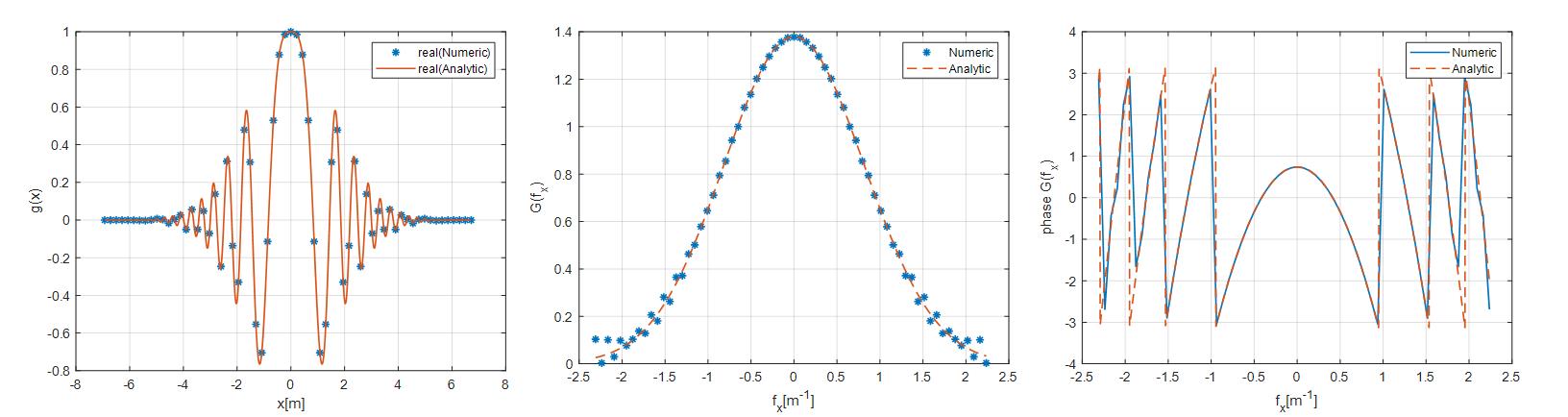
 Note:

(1) The summary of the quadratic phase factor b is as follows: the greater the value of b, the wider the bandwidth of the spectral amplitude of the Gaussian function with the quadratic phase factor;

(2) The value of p can be 1/e^2 = 0.1353 or smaller, such as 0.01 or 0.001. The smaller the value of p, the more accurate DFT can be obtained. When the value of p is too large, it is easy to see aliasing at the high frequency of the spectrum after DFT.