(I've just started to study in depth and try to record all the exercises of the class. I'll give you a dish and chicken. If there is any mistake or lack of understanding, please give me advice.)
2. Preparatory knowledge
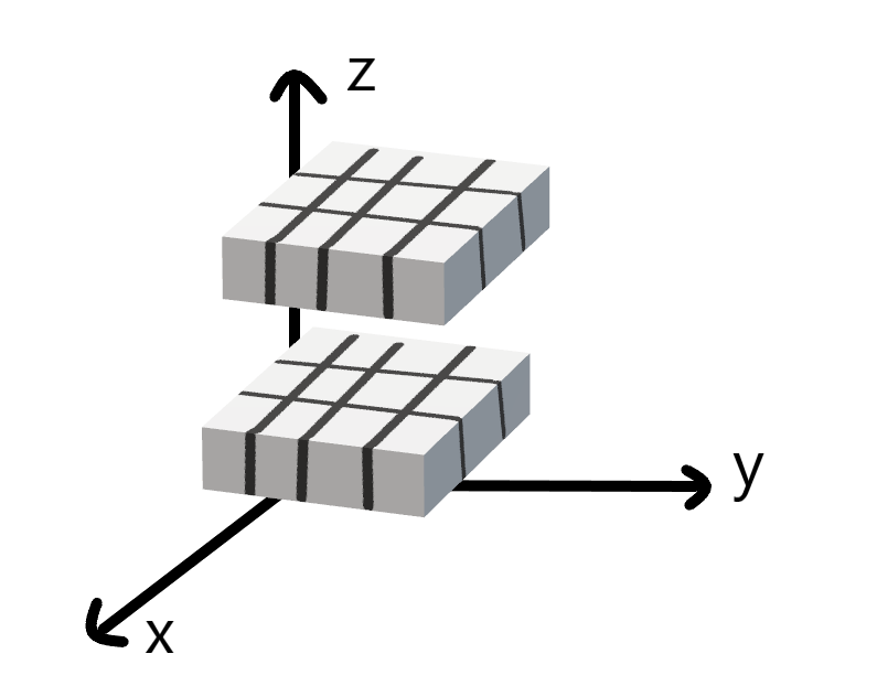
2.1 data operation
First question
Run the code in this section. Change the conditional statement X == Y in this section to x < y or x > y, and then see what kind of tensor you can get
X = torch.arange(12, dtype=torch.float32).reshape((3,4))
Y = torch.tensor([[2.0, 1, 4, 3], [1, 2, 3, 4], [4, 3, 2, 1]])
X < Y, X > Y
Operation results
	(tensor([[ True, False,  True, False],
         [False, False, False, False],
         [False, False, False, False]]),
    tensor([[False, False, False, False],
         [ True,  True,  True,  True],
         [ True,  True,  True,  True]]))
Second question
Replace the two tensors operated by elements in the broadcast mechanism with other shapes, such as three-dimensional tensors. Is the result the same as expected?
If it is (2x1x3) + (1x3x2), an error is reported
a = torch.tensor([[[1,2,3]],[[5,3,5]]])  # 2x1x3
b = torch.tensor([[[1,2],[3,5],[6,7]]])  # 1x3x2
a + b
---------------------------------------------------------------------------
RuntimeError                              Traceback (most recent call last)
Input In [103], in <module>
      1 a = torch.tensor([[[1,2,3]],[[5,3,5]]])
      2 b = torch.tensor([[[1,2],[3,5],[6,7]]])
----> 3 a + b

RuntimeError: The size of tensor a (3) must match the size of tensor b (2) at non-singleton dimension 2
If (1x2x3) + (2x1x3)
a = torch.tensor([[[1, 2, 3], [4, 5, 6]]])  # 1x2x3
b = torch.tensor([[[7, 8, 9]], [[4, 5, 6]]])  # 2x1x3
a + b
The result is (2x2x3)
tensor([[[ 8, 10, 12],
         [11, 13, 15]],

        [[ 5,  7,  9],
         [ 8, 10, 12]]])
about Broadcasting mechanism , refer to the explanation given by pytorch official:
1. Each tensor has at least one dimension.
2. When iterating dimension size, starting from the trailing dimension, the dimension size must be equal, one of which is 1, or one of which does not exist.
An article on "Dog King" was found in the station, which explained in great detail:
Premise 2: look at each dimension of the two tensors in order, and the corresponding two dimensions of x and y need to be able to match. Under what circumstances is it a match? If the following conditions are met:
if these two dimensions are equal in size
elif a dimension has a tensor and a tensor does not
elif has a tensor and a tensor in a certain dimension, but the size is 1
2.2 data preprocessing
os.makedirs(dir_name2, exist_ok=True) can create folders recursively
exist_ When the OK parameter is True, it is judged that if the folder exists, it will not be created
os.path.join() splice file path
First question
Create a raw dataset with more rows and columns. (1) Delete the column with the most missing values. (2) The preprocessed data set is converted to tensor format.
import os
import pandas as pd
import torch

os.makedirs(os.path.join('..', '2.1', 'data2'), exist_ok=True)
data_file = os.path.join('..', '2.1', 'data2', 'house_tiny.csv')
with open(data_file, 'w') as f:
    f.write('NumRooms,Alley,Floor,Price\n')
    f.write('NA,Pave,2,127500\n')
    f.write('2,NA,1,106000\n')
    f.write('4,NA,NA,178100\n')
    f.write('NA,NA,2,140000\n')
    f.write('NA,NA,2,152000\n')
data = pd.read_csv(data_file)
inputs, outputs = data.iloc[:, 0:3], data.iloc[:, 3]

num = inputs.isnull().sum() # Get the maximum number of missing values
Max_NaN = inputs.isnull().sum().idxmax()  # Gets the index of the maximum number of missing values
inputs = inputs.drop(Max_NaN, axis=1) # Delete the item with the most missing value in inputs
inputs = inputs.fillna(inputs.mean()) # Replace the missing items of the same column with the mean of the same column
inputs = pd.get_dummies(inputs, dummy_na=True)

x, y = torch.tensor(inputs.values), torch.tensor(outputs.values)  # Into tensor form
Operation results
(tensor([[3.0000, 2.0000],
         [2.0000, 1.0000],
         [4.0000, 1.7500],
         [3.0000, 2.0000],
         [3.0000, 2.0000]], dtype=torch.float64),
 tensor([127500, 106000, 178100, 140000, 152000]))
df.isnull().sum() count the null value of the number of rows in each column and return the number of rows
. idxmax() get the index corresponding to the maximum value of series in pandas.
The drop function deletes rows by default, and axis = 1 should be added to columns
2.3 linear algebra
First question
It is proved that the transpose of a matrix A is a, that is, (AT)T=A
A = torch.randn(4, 3)
A == A.T.T
Operation results
tensor([[True, True, True],
        [True, True, True],
        [True, True, True],
        [True, True, True]])
Second question
Two matrices A and B are given, and it is proved that "the sum of their transposes" is equal to "the transpose of their sums", that is, AT+BT=(A+B)T
A = torch.arange(12).reshape(3,4)
B = torch.randn(3,4)
A.T + B.T == (A + B).T
Operation results
tensor([[True, True, True],
        [True, True, True],
        [True, True, True],
        [True, True, True]])
Question 3
Given an arbitrary square matrix A, is A+AT always symmetric? Why?
A = torch.randn(4, 4)
(A + A.T).T == (A + A.T)
Operation results
tensor([[True, True, True, True],
        [True, True, True, True],
        [True, True, True, True],
        [True, True, True, True]])
Question 4
In this section, we define the tensor X of shape (2,3,4). What is the output of len(X)?
X = torch.arange(24).reshape(2, 3, 4)
len(X)
Operation results
2
Question 5
For tensor X of any shape, does len (x) always correspond to the length of a specific axis of X? What is this axis?
X = torch.arange(24).reshape(2, 3, 4)  # 2x3x4 tensor
Y = torch.arange(24).reshape(4, 6)  # 4X6 tensor
Z = torch.ones(1)   # One dimensional tensor
len(X), len(Y), len(Z)
Operation results
2 4 6
len() returns the length of the zeroth dimension of the tensor
Question 6
Run A / A.sum(axis=1) to see what happens. Can you analyze the reason?
- If A is A square matrix
A = torch.arange(16).reshape(4, 4)  # 4X4
A / A.sum(axis=1)
Operation results
tensor([[0.0000, 0.0455, 0.0526, 0.0556],
        [0.6667, 0.2273, 0.1579, 0.1296],
        [1.3333, 0.4091, 0.2632, 0.2037],
        [2.0000, 0.5909, 0.3684, 0.2778]])
- If A is not A square matrix
A = torch.arange(12).reshape(3, 4)  # 3X4
B = torch.arange(12).reshape(4, 3)  # 4x3
A / A.sum(axis=1)  # Or B / B.sum(axis=1)
Operation results
RuntimeError                              Traceback (most recent call last)
Input In [78], in <module>
----> 1 A / A.sum(axis=1)

RuntimeError: The size of tensor a (4) must match the size of tensor b (3) at non-singleton dimension 1
If a is a square matrix and A.sum(axis=1) is dimension reduction along the 1 axis, the result is equal to the length of a matrix, and the matrix can be divided by elements
If a is not a square matrix, A.sum(axis=1) reduces the dimension along the 1 axis, and the result is not equal to the length of a matrix, so it cannot be calculated according to elements
Question 7
Considering a tensor with shape (2,3,4), what is the shape of the summation output on axes 0, 1 and 2?
A = torch.arange(24).reshape(2,3,4)  # 2x3x4
A.sum(axis=0).shape, A.sum(axis=1).shape, A.sum(axis=2).shape
Operation results
torch.Size([3, 4])
torch.Size([2, 4])
torch.Size([2, 3])
Question 8
Is linalg The norm function provides tensors of three or more axes and observes their output. What does this function calculate for tensors of any shape?
A, B = torch.randn(2,3,4), torch.randn(3, 4)
outputs1 = torch.linalg.norm(A)  # 2x3x4 tensor
outputs2 = torch.linalg.norm(B)  # 3x4 tensor
A, B, outputs1, outputs2
Operation results
(tensor([[[ 2.1417, -1.2939, -0.0506,  0.0582],
          [ 0.9437,  0.3785, -0.0736, -0.1000],
          [-0.2323,  1.3399,  0.6603,  0.8154]],

         [[-0.1303, -0.4355, -0.2770,  1.8112],
          [ 0.7443, -0.1177,  0.8033,  0.0264],
          [ 0.5158, -0.1448, -0.7694, -0.5072]]]),
 tensor([[-1.1264,  0.0546,  0.4413, -0.1869],
         [-1.7601, -0.4381, -0.2288, -1.7541],
         [-0.1453,  1.0307, -0.8918,  0.7459]]),
 tensor(4.0225),
 tensor(3.2180))
Equivalent to finding L2 norm, which can represent the size of tensor
2.4 calculus
First question
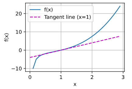
Draw function y = f ( x ) = x 3 − 1 x y=f(x)=x^{3}-\frac{1}{x} y=f(x)=x3 − x1 and its x = 1 x=1 The image of the tangent at x=1.
plot(x, [x ** 3 - 1 / x, 4 * x - 4], 'x', 'f(x)', legend=['f(x)', 'Tangent line (x=1)'])
Operation results
Second question
Find function f ( x ) = 3 x 1 2 + 5 e x 2 f(x)=3x_{1}^{2}+5e^{x_{2}} F (x) = gradient of 3x12 + 5ex2.
[ 6 x 1 6x_{1} 6x1, 5 e x 2 5e^{x_{2}} 5ex2] derive x1 of the first term and x2 of the second term respectively the gradient is in vector form
Question 3
function f ( x ) = ∥ x ∥ 2 f(x)=\left \| x \right \|_{2} What is the gradient of f(x) = ‖ x ‖ 2?
∂ f ( x ) ∂ x = ∂ ∥ x ∥ 2 ∂ x = x ∥ x ∥ 2 \frac{\partial f(x)}{\partial x}=\frac{\partial \left \| x \right \|_{2}}{\partial x}=\frac{x}{\left \| x \right \|_{2}} ∂x∂f(x)=∂x∂∥x∥2=∥x∥2x
L2 norm can be regarded as x 2 \sqrt{x^{2}} x2 , then f ( x ) f(x) f(x) gradient is x 2 \sqrt{x^{2}} x2 Right x x x derivative: f ′ ( x ) = 2 x 2 x 2 = x x 2 = x ∥ x ∥ 2 f^{'}(x)=\frac{2x}{2\sqrt{ x^{2}}}=\frac{x}{\sqrt{x^{2}}}=\frac{x}{\left \| x \right \|_{2}} f′(x)=2x2 2x=x2 x=∥x∥2x
Question 4
You can write functions u = f ( x , y , z ) u=f(x,y,z) u=f(x,y,z), where x = x ( a , b ) x=x(a,b) x=x(a,b) , y = y ( a , b ) y=y(a,b) y=y(a,b), z = z ( a , b ) z=z(a,b) Z = the chain rule of Z (a, b)?
d
u
d
a
=
d
u
d
x
d
x
d
a
+
d
u
d
y
d
y
d
a
+
d
u
d
z
d
z
d
a
\frac{du}{da}=\frac{du}{dx}\frac{dx}{da}+\frac{du}{dy}\frac{dy}{da}+\frac{du}{dz}\frac{dz}{da}
dadu=dxdudadx+dydudady+dzdudadz
d
u
d
b
=
d
u
d
x
d
x
d
b
+
d
u
d
y
d
y
d
b
+
d
u
d
z
d
z
d
b
\frac{du}{db}=\frac{du}{dx}\frac{dx}{db}+\frac{du}{dy}\frac{dy}{db}+\frac{du}{dz}\frac{dz}{db}
dbdu=dxdudbdx+dydudbdy+dzdudbdz
2.5 automatic differentiation
requires_grad is an attribute of Tensor, a general data structure in pytoch, which is used to indicate whether the current quantity needs to retain the corresponding gradient information in the calculation
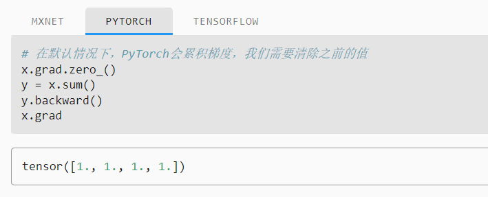
The summation of vector x is equivalent to multiplying the vector by a unit vector E, so the gradient is 1
First question
Why is it more expensive to calculate the second derivative than the first derivative?
Because to calculate the second-order reciprocal, you need to calculate the first derivative first
Second question
Immediately after running the back propagation function, run it again to see what happens.
import torch

x = torch.arange(4.0, requires_grad=True)
y = 2 * torch.dot(x, x)
y.backward()
y.backward()  # Perform another backpropagation now
x.grad
Operation results
RuntimeError: Trying to backward through the graph a second time, but the saved intermediate results have already been freed. Specify retain_graph=True when calling .backward() or autograd.grad() the first time. # When trying the second back propagation, the result of the first back propagation has been released
For the first time When backward, specify retain graph=True
import torch

x = torch.arange(4.0, requires_grad=True)
y = 2 * torch.dot(x, x)
y.backward(retain_graph=True)  # The reserved calculation chart is not released
y.backward()
x.grad
Operation results
tensor([ 0., 8., 16., 24.])
By default, pytorch cannot continuously perform back propagation. If line sequence execution is required, x.grad needs to be updated
Question 3
In the control flow example, we calculate the derivative of d with respect to A. what happens if we change the variable a to a random vector or matrix?
import torch

def f(a):
    b = a * 2
    while b.norm() < 1000:
        b = b * 2
    if b.sum() > 0:
        c = b
    else:
        c = 100 * b
    return c

a = torch.randn(size=(2,2), requires_grad=True)  # a is 2x2
d = f(a)
d.backward()
Operation results
RuntimeError: grad can be implicitly created only for scalar outputs # No back propagation of vectors or matrices
For non scalars (vectors or matrices), you need to specify that the length of the gradient matches its length
Question 4
Redesign an example of finding the gradient of control flow, run and analyze the results.
import torch

def f(a):
    b = a / 2
    while b > 1:
        b = pow(a, 2)
    if b < 3:
        c = b * 2
    else:
        c = b * 3
    return c

a = torch.randn(size=(), requires_grad=True)
d = f(a)
d.backward()
a.grad == d / a
Operation results
tensor(True)
Consistent with the example ideas in 2.5.4
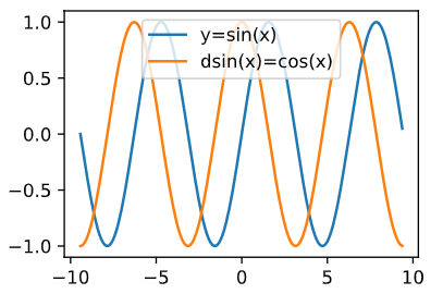
Question 5
send f ( x ) = s i n ( x ) f(x)=sin(x) f(x)=sin(x), plot f ( x ) f(x) f(x) and d f ( x ) d x \frac{df(x)}{dx} dxdf(x), where the latter is not used f ′ ( x ) = c o s ( x ) f^{'}(x)=cos(x) f′(x)=cos(x)
error code
import torch
import matplotlib.pyplot as plt
import numpy as np
x = torch.arange(-3*np.pi, 3*np.pi, 0.1,requires_grad=True)
y = torch.sin(x)

y.sum().backward()

plt.plot(x, y, label='y=sin(x)')
plt.plot(x, x.grad, label='dsin(x)=cos(x)')
plt.legend(loc='upper center')
plt.show()
report errors:
RuntimeError: Can't call numpy() on Tensor that requires grad. Use tensor.detach().numpy() instead.
You cannot call numpy() on a tensor to grad and apply tensor detach(). Numpy() instead
error code
y.backward()
report errors:
grad can be implicitly created only for scalar outputs
When y is a scalar, back propagation can be carried out, and each input x corresponds to a scalar output y *, so a scalar can be obtained by using y.sum
import torch
import matplotlib.pyplot as plt
import numpy as np
x = torch.arange(-3*np.pi, 3*np.pi, 0.1,requires_grad=True)
y = torch.sin(x)

y.sum().backward()

plt.plot(x.detach(), y.detach(), label='y=sin(x)')
plt.plot(x.detach(), x.grad, label='dsin(x)=cos(x)')
plt.legend(loc='upper center')
plt.show()
Operation results
2.6 probability
%matplotlib inline is magic functions: IPython has a set of pre-defined so-called magic functions that can be accessed through the syntax of the command line. "%" is followed by the parameters of the magic function
The function of this function is embedded drawing, and PLT is omitted show()
torch.cumsum(input, dim, *, dtype=None, out=None) returns the cumulative sum of input elements in dimension dim
First question
m=500 groups of experiments were carried out, and n=10 samples were taken from each group. Change m and n, observe and analyze the experimental results.
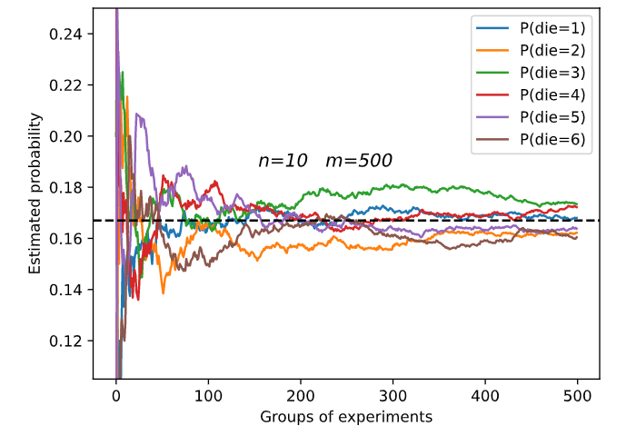
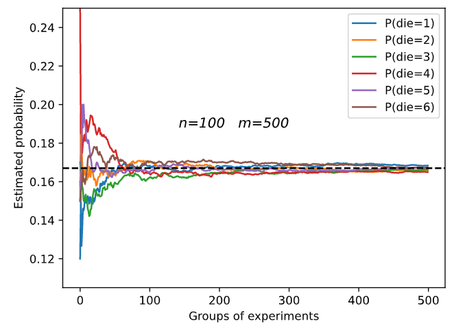
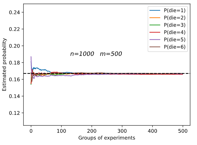
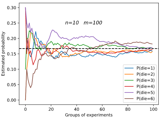
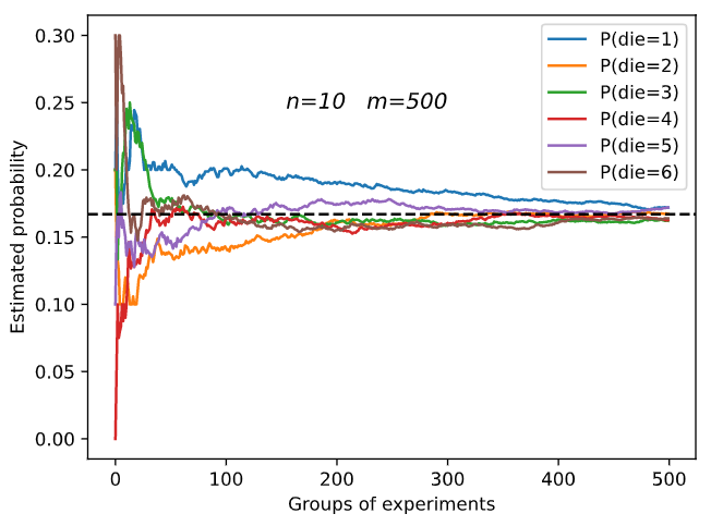
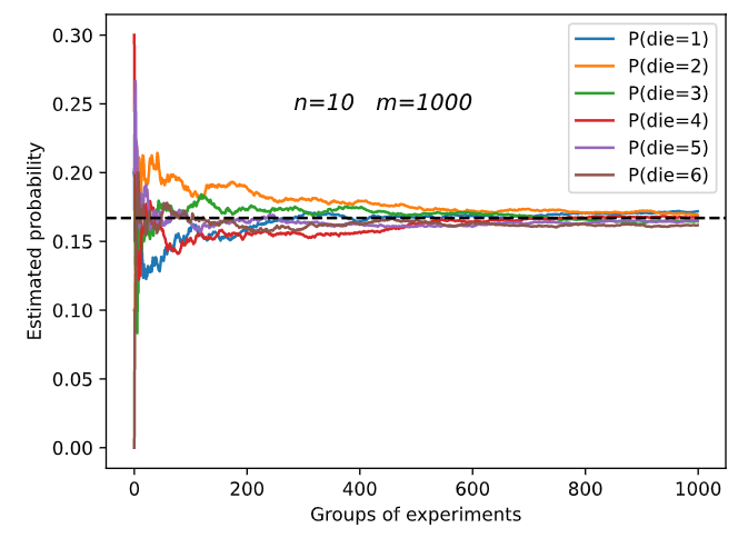
Increasing m or n will increase the sample size, which will make the result tend to the real probability
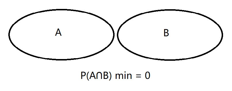
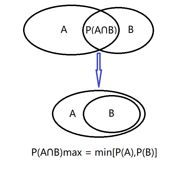
Second question
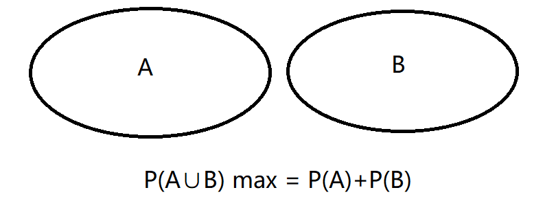
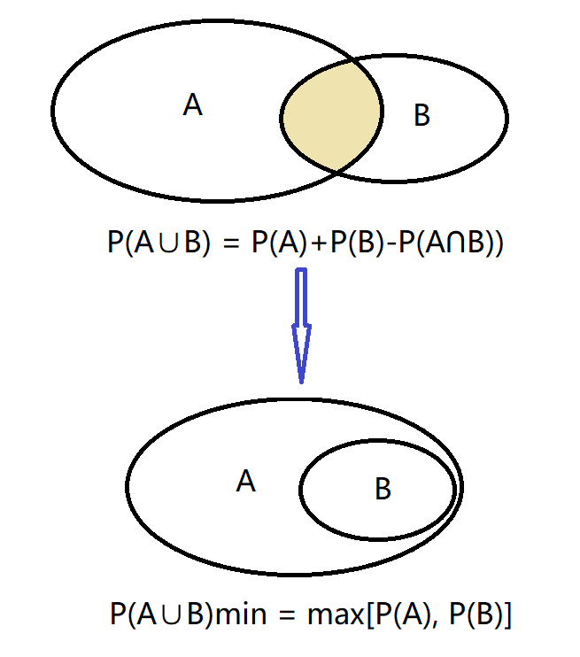
Given two events with probability P(A) and P(B), calculate the upper and lower limits of P(A ∪ B) and P(A ∩ B).
Question 3
Suppose we have A series of random variables, such as A, B and C, where B only depends on A and C only depends on B. can you simplify the joint probability P(A,B,C)?
Markov chain is a set of discrete random variables with Markov properties. Specifically, for probability space ( ℧ , F , P ) (\mho ,F,\mathbb{P}) A set of random variables in (℧, F,P) with one-dimensional countable set as index set X = { X n : n > 0 } X=\left \{ X_{n}:n>0 \right \} X={Xn: n > 0}, if the values of random variables are in the countable set: X = s i , s i ∈ s X=s_{i},s_{i}\in s X=si, si ∈ s, and the conditional probability of random variables satisfies the following relationship: P ( X t + 1 ∣ X t , . . . , X 1 ) = P ( X t + 1 ∣ X t ) P(X_{t+1}|X_{t},...,X_{1})=P(X_{t+1}|X_{t}) P(Xt+1∣Xt,...,X1)=P(Xt+1∣Xt)
P ( A B C ) = P ( A ) P ( B ∣ A ) P ( C ∣ B A ) = P ( A ) P ( B ∣ A ) P ( C ∣ B ) P(ABC)=P(A)P(B|A)P(C|BA)=P(A)P(B|A)P(C|B) P(ABC)=P(A)P(B∣A)P(C∣BA)=P(A)P(B∣A)P(C∣B)

See P7, 4 of Zhang Yu's 9 lectures on probability theory and mathematical statistics, 2022 edition notes
Question 4
In section 2.6.2.6, the first test is more accurate. Why not run the first test twice, but run the first and second tests at the same time?
Because the characteristics of each test are different, each test will be affected differently. If you run the first test twice, this impact will be superimposed. Running the first and second tests at the same time can effectively offset this impact.