Reading notes of Python deep learning: Chapter 2 mathematical basis of neural network

# Load MNIST dataset in Keras
from keras.datasets import mnist
(train_images, train_labels), (test_images, test_labels) = mnist.load_data()


print(train_images.shape)
print(len(train_labels))
print(train_labels)

print(test_images.shape)
print(len(test_labels))
print(test_labels)

(60000, 28, 28)
60000
[5 0 4 ... 5 6 8]
(10000, 28, 28)
10000
[7 2 1 ... 4 5 6]

The following work flow is as follows: firstly, the training data (train_images and train_labels) are input into the neural network; Secondly, web-based learning associates images and labels together; Finally, the network pair test_images generates predictions, which we will verify with test_ Whether the labels in labels match.

The core component of neural network is layer, which is a data processing module. You can regard it as a data filter, put in some data, and the resulting data becomes more useful. Specifically, the layer extracts representations from the data -- and we expect such representations to help solve the problem at hand. Most deep learning is to link simple layers to achieve progressive data distillation. The deep learning model is like a sieve of data processing, including a series of increasingly fine data filters (i.e. layers).

To train the network, we also need to select the three parameters of the compilation step.

1. Loss function: how to measure the performance of the network on the training data, that is, how the network moves in the right direction;

2. Optimizer: a mechanism to update the network based on training data and loss function;

3. Indicators to be monitored during training and testing: this example only cares about accuracy, that is, the proportion of correctly classified images.

from keras import models
from keras import layers

network = models.Sequential()
network.add(layers.Dense(512, activation='relu', input_shape=(28 * 28,)))
network.add(layers.Dense(10, activation='softmax'))
network.compile(optimizer='rmsprop', loss='categorical_crossentropy', metrics=['accuracy'])

Before training, we will preprocess the data, transform it into the shape required by the network, and shrink it to the range where all values are in [0,1].

train_images = train_images.reshape((60000, 28 * 28))
train_images = train_images.astype('float32') / 255

test_images = test_images.reshape((10000, 28 * 28))
test_images = test_images.astype('float32') / 255

We also need to classify and code the labels.

from keras.utils.np.utils import to_categorical

train_labels = to_categorical(train_labels)
test_labels = to_categorical(test_labels)

Now we are ready to start training the network. In Keras, this step is completed by calling the fit method of the network - we fit the model on the training data.

print(network.fit(train_images, train_labels, epochs=5, batch_size=128))

Epoch 1/5
469/469 [==============================] - 3s 4ms/step - loss: 0.2583 - accuracy: 0.9255
Epoch 2/5
469/469 [==============================] - 2s 4ms/step - loss: 0.1044 - accuracy: 0.9688
Epoch 3/5
469/469 [==============================] - 2s 4ms/step - loss: 0.0691 - accuracy: 0.9796
Epoch 4/5
469/469 [==============================] - 2s 4ms/step - loss: 0.0500 - accuracy: 0.9848
Epoch 5/5
469/469 [==============================] - 2s 4ms/step - loss: 0.0379 - accuracy: 0.9884

Two numbers are displayed in the training process: one is the loss of the network in the training data, and the other is the accuracy of the network in the training data. We quickly achieved 98.8% accuracy in the training data. Now let's check the performance of the model on the test set.

test_loss, test_acc = network.evaluate(test_images, test_labels)
print('test_acc:', test_acc)

test_acc: 0.9794999957084656

The accuracy of the test set is 97.9%, which is much lower than that of the training set. The gap between training accuracy and testing accuracy is caused by over fitting, which means that the performance of machine learning model on new data is often worse than that on training data.

2.2 data representation of neural network

The data used in the previous example is stored in a multidimensional Numpy array, also known as tensor. Generally speaking, all current machine learning systems use tensors as the basic data structure. The core of the concept of tensor is that it is a data container. The data it contains is almost always numerical data, so it is a container of numbers. Matrix is a two-dimensional tensor, which is the generalization of matrix to any dimension. The dimension of tensor is usually called axis.

2.2.1 scalar (0D tensor)

Tensors that contain only one number are called scalars (also known as scalar tensors, zero dimensional tensors, 0D tensors). In Numpy, a number of float32 or float64 is a scalar tensor (or scalar array). Scalar tensors have 0 axes (ndim == 0), and the number of tensor axes is also called order.

import numpy as np

x = np.array(12)
print(x)
print(x.ndim)

12
0

2.2.2 vector (1D tensor)

An array of numbers is called a vector or one-dimensional tensor (1D tensor). One dimensional tensor has only one axis.

x = np.array([12, 3, 6, 14, 7])
print(x)
print(x.ndim)

[12  3  6 14  7]
1

2.2.3 matrix (2D tensor)

An array of vectors is called a matrix or two-dimensional tensor (2D tensor). A matrix has two axes (usually called rows and columns). You can intuitively understand a matrix as a rectangular grid of numbers.

x = np.array([[5, 78, 2, 34, 0],
              [6, 79, 3, 35, 1],
              [7, 80, 4, 36, 2]])
print(x)
print(x.ndim)

[[ 5 78  2 34  0]
 [ 6 79  3 35  1]
 [ 7 80  4 36  2]]
2

The elements on the first axis are called rows, and the elements on the second axis are called columns.

2.2.4 3D tensor and higher dimensional tensor

Combining multiple matrices into a new array can get a 3D tensor, which you can intuitively understand as a cube composed of numbers.

x = np.array([[[5, 78, 2, 34, 0],
               [6, 79, 3, 35, 1],
               [7, 80, 4, 36, 2]],
              [[5, 78, 2, 34, 0],
               [6, 79, 3, 35, 1],
               [7, 80, 4, 36, 2]],
              [[5, 78, 2, 34, 0],
               [6, 79, 3, 35, 1],
               [7, 80, 4, 36, 2]]])
print(x)
print(x.ndim)

[[[ 5 78  2 34  0]
  [ 6 79  3 35  1]
  [ 7 80  4 36  2]]

 [[ 5 78  2 34  0]
  [ 6 79  3 35  1]
  [ 7 80  4 36  2]]

 [[ 5 78  2 34  0]
  [ 6 79  3 35  1]
  [ 7 80  4 36  2]]]
3

Combining multiple 3D tensors into an array can create a 4D tensor, and so on. The tensor of deep learning processing is generally 0D to 4D, but 5D tensor may be encountered when processing video data.

2.2.5 key attributes

Tensors are defined by the following three key attributes.

1. Number of shafts (order). The 3D tensor has three axes and the matrix has two axes.

2. Shape. This is an integer tuple that represents the dimension size (number of elements) of the tensor along each axis.

3. Data type. This is the type of data contained in the tensor. For example, the type of tensor can be float32, unit8, float64, etc. In rare cases, you may encounter character tensors. String tensors do not exist in Numpy (and most other libraries) because tensors are stored in pre allocated contiguous memory segments, and the length of strings is variable and cannot be stored in this way.

from keras.datasets import mnist

(train_images, train_labels), (test_images, test_labels) = mnist.load_data()

print(train_images.ndim)
print(train_images.shape)
print(train_images.dtype)

3
(60000, 28, 28)
uint8

So, here's train_images is a 3D tensor composed of 8-bit integers. More specifically, it is an array composed of 60000 matrices. Each matrix is composed of 28x28 integers. Each such matrix is a gray image, and the value range of elements is 0 ~ 255.

import matplotlib.pyplot as plt

digit = train_image[3]
plt.imshow(digit, cmap=plt.cm.binary)
plt.show()

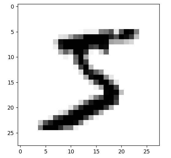
The figure above shows the fourth sample in the dataset.

2.2.6 manipulating tensors in Numpy

In the previous example, we used the syntax train_images[i] to select a specific number along the first axis, and the specific element of the selected tensor is called tensor slice.

my_slice = train_images[9:99]
print(my_slice.shape)

(90, 28, 28)

In the above example, select the 10th to 100th numbers (excluding the 100th) and put them in the array with shape (90, 28, 28).

It is equivalent to the following more complex formulation, which gives the start index and end index of the slice along each tensor axis: Equivalent to selecting the entire axis.

my_slice = train_images[9:99, :, :]
print(my_slice.shape)

my_slice = train_images[9:99, 0:28, 0:28]
print(my_slice.shape)

2.2.7 concept of data batch

Generally speaking, the first axis of all data tensors in deep learning (0 axis, because the index starts from 0) is the sample axis (sometimes called the sample dimension).

In addition, the deep learning model will not process the whole data set at the same time, but split the data into small batches.

batch = train_images[:128]
batch = train_images[128:256]
batch = train_images[128 * n:128 * (n + 1)]

For this batch tensor, the first axis (0 axis) is called batch axis or batch dimension.

2.2.8 data tensor in the real world

1. Vector data: 2D tensor;

2. Time series data or series data: 3D tensor;

3. Image: 4D tensor;

4. Video: 5D tensor.

2.2.9 vector data

This is the most common data. For this data set, each data point is encoded as a vector, so a data batch is encoded as a 2D tensor (i.e. an array of vectors), in which the first axis is the sample axis and the second axis is the characteristic axis.

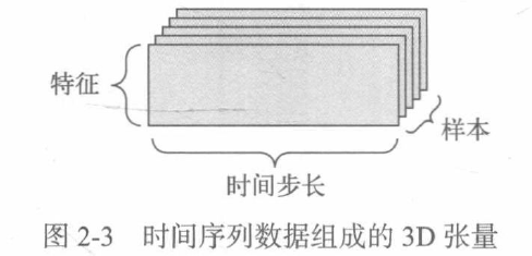
2.2.10 time series data or series data

When time (or sequence order) is important to data, the data should be stored in 3D tensor with time axis. Each sample can be encoded as a vector sequence (i.e. 2D tensor), so a data batch is encoded as a 3D tensor.

2.2.11 image data

Images usually have three dimensions: height, width and color depth. Although the gray-scale image has only one color channel, so it can be saved in 2D tensor, according to convention, the image tensor is always 3D tensor, and the color channel of gray-scale image is only one-dimensional.

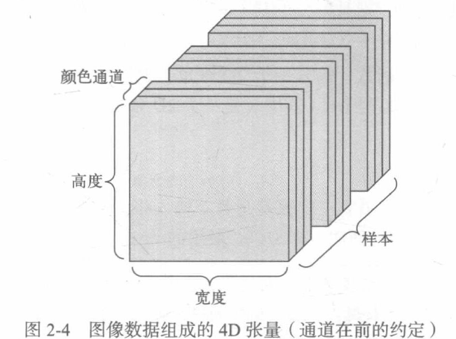
There are two conventions for the shape of image tensor: the Convention of channel in the back and the Convention of channel in the front.

2.2.12 video data

Video data is one of the few data types that need 5D tensor in real life. Video can be regarded as a series of frames, and each frame is a color image. Since each frame can be saved in a 3D tensor, a series of frames can be saved in a 4D tensor, while batch frames composed of different videos can be saved in a 5D tensor.

2.3 "gear" of neural network: tensor operation

All computer programs can eventually be simplified into some binary operations on binary input. Similarly, all transformations learned by deep neural network can also be simplified into some tensor operations on numerical data tensor.

In the initial example, we built the network by overlaying the density layer.

2.3.1 element by element operation

Both relu operation and addition are element by element operation, that is, the operation is applied to each element in the tensor independently, that is, these operations are very suitable for large-scale parallel implementation (vectorization Implementation)

def naive_relu(x):
    assert len(x.shape) == 2
    
    x = x.copy()
    for i in range(x.shape[0]):
        for j in range(x.shape[1]):
            x[i, j] = max(x[i, j], 0)
    
    return x


def naive_add(x, y):
    assert len(x.shape) == 2
    assert x.shape == y.shape
    
    x = x.copy()
    for i in range(x.shape[0]):
        for j in range(x.shape[1]):
            x[i, j] += y[i, j]
    
    return x

2.3.2 broadcasting

If there is no ambiguity, the smaller tensor will be broadcast to match the shape of the larger tensor. The broadcast includes the following two steps:

1. Add an axis (called broadcast axis) to the smaller tensor to make its ndim the same as the larger tensor;

2. Repeat the smaller tensor along the new axis to make its shape the same as the larger tensor.

def naive_add_matrix_and_vector(x, y):
    assert len(x.shape) == 2
    assert len(y.shape) == 1
    assert x.shape[1] == y.shape[0]
    
    x = x.copy()
    for i in range(x.shape[0]):
        for i in range(x.shape[1]):
            x[i, j] += y[j]
    
    return x

The following example uses broadcast to apply the element by element maximum operation to two tensors with different shapes.

import numpy as np

x = np.random.random((64, 3, 32, 10))
y = np.random.random((32, 10))

z = np.maximum(x, y)

2.3.3 tensor dot product

Dot product operation, also known as tensor product (don't confuse it with element by element product), is the most common and useful tensor operation. Unlike the element by element operation, it combines the elements of the input tensor.

Let's first look at the dot product of two vectors x and y, and its calculation process is as follows:

def naive_vector_dot(x, y):
    assert len(x.shape) == 1
    assert len(y.shape) == 1
    assert x.shape[0] == y.shape[0]
    
    z = 0
    for i in range(x.shape[0]):
        z += x[i] * y[i]
    
    return z

The dot product between two vectors is a scalar, and only vectors with the same number of elements can be dot products.

A matrix x and a vector y do dot product, and the return value is a vector, where each element is the dot product between each row of Y and x.

import numpy as np


def naive_matrix_vector_dot(x, y):
    assert len(x.shape) == 2
    assert len(y.shape) == 1
    assert x.shape[1] == y.shape[0]
    
    z = np.zeros(x.shape[0])
    for i in range(x.shape[0]):
        for j in range(x.shape[1]):
            z[i] += x[i, j] * y[j]
    
    return z

def naive_matrix_vector_dot(x, y):
    z = np.zeros(x.shape[0])
    for i in range(x.shape[0]):
        z[i] = naive_vector_dot(x[i, :], y)

    return z

If the ndim of one of the two tensors is greater than 1, the dot operation is no longer symmetrical, that is, dot(x, y) is not equal to dot(y, x).

The point product can be extended to tensors with any axis. The most common application may be the point product between two matrices. For two matrices X and y, you can do the point product (dot(x, y)) only when x.shape[1] == y.shape[0]). The result is a matrix with shape (x.shape[0], y.shape[1]), whose element is the dot product between the row of X and the column of Y.

def naive_matrix_dot(x, y):
    assert len(x.shape) == 2
    assert len(y.shape) == 2
    assert x.shape[1] == y.shape[0]

    z = np.zeros((x.shape[0], y.shape[1]))
    for i in range(x.shape[0]):
        for j in range(y.shape[1]):
            row_x = x[i, :]
            column_y = y[:, j]
            z[i, j] = naive_vector_dot(row_x, column_y)

    return z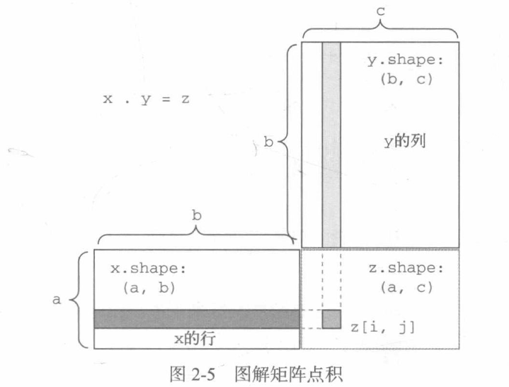

As shown in the figure, x, y and z are represented by rectangles (elements are arranged in rectangles). The rows of X and the columns of y must be the same size, so the width of X must be equal to the height of Y.

2.3.4 tensor deformation

The third important tensor operation is tensor deformation. We use this operation in preprocessing before inputting image data into neural network.

Tensor deformation refers to changing the rows and columns of tensor to get the desired shape. The total number of elements of the deformed tensor is the same as that of the initial tensor.

import numpy as np


x = np.array([[0., 1.],
              [2., 3.],
              [4., 5.]])
print(x)

x = x.reshape((6, 1))
print(x)

x = x.reshape((2, 3))
print(x)

[[0. 1.]
 [2. 3.]
 [4. 5.]]
[[0.]
 [1.]
 [2.]
 [3.]
 [4.]
 [5.]]
[[0. 1. 2.]
 [3. 4. 5.]]

A special tensor deformation often encountered is transposition. Transposition of a matrix refers to the exchange of rows and columns, so that x[i,:] becomes x[:, i].

x = np.zeros((300, 20))
x = np.transpose(x)
print(x.shape)

(20, 300)

2.3.5 geometric interpretation of tensor operation

For the tensor operated by tensor operation, its elements can be interpreted as the coordinates of points in some geometric space, so all tensor operations have geometric interpretation.

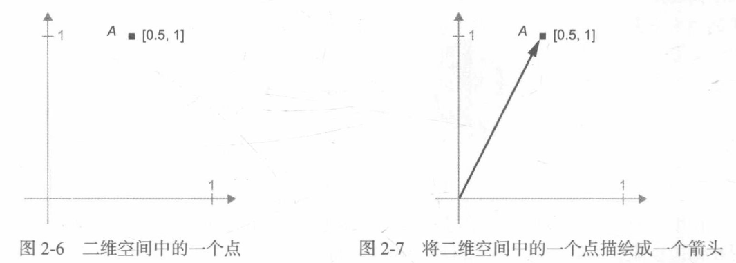
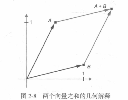
Generally speaking, the basic geometric operations such as affine transformation, rotation and scaling can be expressed as tensor operations.

2.3.6 geometric interpretation of deep learning

Neural network is completely composed of a series of tensor operations, and these tensor operations are only the geometric transformation of input data. Therefore, you can interpret neural networks as very complex geometric transformations in high-dimensional space.

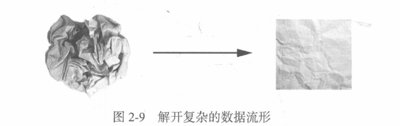
What the neural network (or any machine learning model) needs to do is find the transformation that can restore the flatness of the paper ball, so that the two categories can be clearly divided again. Through deep learning, this process can be realized by a series of simple transformations in three-dimensional space.

Making the paper ball flat is the content of machine learning: finding a concise representation of complex and highly folded data manifolds. Deep learning gradually decomposes the complex geometric transformation into a long series of basic geometric transformations, which is roughly the same as the strategy adopted by human beings to unfold the paper ball. Each layer of the deep network makes the data unravel a little bit through transformation - many layers are stacked together, which can realize a very complex unraveling process.

2.4 "engine" of neural network: gradient based optimization

output = relu(dot(W, input) + b)

In this expression, W and b are tensors, which are the properties of the layer. They are called the weights or trainable parameters of this layer, which correspond to the kernel and bias attributes respectively. These weights contain the information learned by the network from observing the training data.

At first, these weight matrices take small random values. This step is called random initialization. The next step is to gradually adjust these weights according to the feedback signal. This process of gradual adjustment is called training, that is, learning in machine learning.

The above process takes place in a training cycle. The specific process is as follows. Repeat these steps all the time if necessary:

1. Extract the data batch composed of training sample x and corresponding target y;

2. Run the network on x [this step is called forward propagation] to get the predicted value y_pred；

3. Calculate the loss of the network on this batch of data to measure y_ Distance between PRED and Y;

4. Update all weights of the network to reduce the loss of the network on this batch of data slightly.

The loss of the final network on the training data is very small, that is, the predicted value y_ The distance between PRED and the expected target y is very small. The network "learns" to map input to the correct target.

The difficulty lies in the fourth step: update the weight of the network. Considering a weight coefficient in the network, how do you know whether this coefficient should increase or decrease, and how much it changes?

A simple solution is to keep other weights in the network unchanged, only consider a scalar coefficient and let it try different values.

A better method is to take advantage of the fact that all operations in the network are differentiable, calculate the gradient of the loss relative to the network coefficient, and then change the coefficient in the opposite direction of the gradient to reduce the loss.

2.4.1 what is derivative

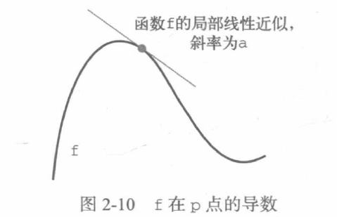
The derivative completely describes how f(x) will change after changing X. if you want to reduce the value of f(x), just move x a small step in the opposite direction of the derivative.

2.4.2 derivative of tensor operation: gradient

Gradient is the derivative of tensor operation. It is the extension of the derivative of multivariate function, which takes tensor as input.

As we have seen before, the derivative of univariate function f(x) can be regarded as the slope of function f curve. Similarly, gradient(f)(W0) can also be regarded as a tensor representing the curvature of f(W) near W0.

For a function f(x), you can reduce the value of f(x) by moving x a small step in the opposite direction of the derivative. Similarly, for the tensor function f(W), you can also reduce f(W) by moving w in the opposite direction of the gradient. That is, moving in the opposite direction of curvature will intuitively lower the position on the curve.

2.4.3 random gradient descent

Given a differentiable function, its minimum value can be found analytically in theory: the minimum value of the function is the point with derivative 0, so you just need to find all points with derivative 0, and then calculate which point of the function has the minimum value.

Applying this method to neural network is to use analytical method to find the ownership weight corresponding to the minimum loss function.

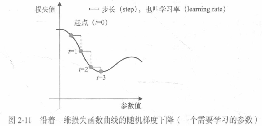
The weight is updated in the opposite direction of the gradient, and the loss decreases a little each time.

1. Extract the data batch composed of training sample x and corresponding target y;

2. Run the network on x to get the predicted value y_pred；

3. Calculate the loss of the network on this batch of data;

4. Move the parameter along the opposite direction of the gradient, such as W -= step * gradient, so as to reduce the loss of this batch of data.

This method is called small batch random gradient descent, also known as small batch SDG. The term random means that each batch of data is randomly selected.

A variant of small batch SGD algorithm is to extract only one sample and target at each iteration, rather than a batch of data, which is called true SGD (different from small batch SGD). At the other extreme, each iteration runs on all data, which is called batch SGD. In this way, each update is more accurate, but the calculation cost is much higher. The effective compromise between the two extremes is to choose a reasonable batch size.

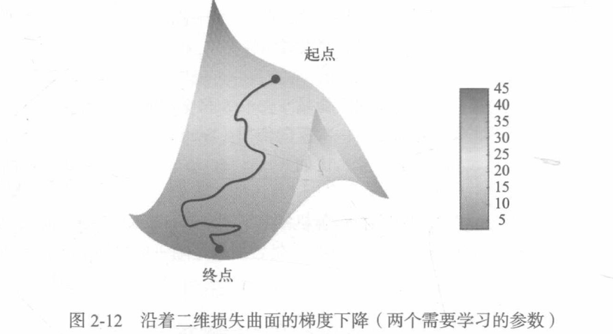
Each weight parameter of neural network is a free dimension in space, and the network may contain tens of thousands or even millions of parameter dimensions. You can't visualize the actual training process of neural network, because you can't visualize 1000000 dimensional space in a way that humans can understand. Therefore, it is best to remember that the intuition formed in these low dimensional representations is not always accurate in practice, which has been the source of problems in deep learning research in history.

In addition, there are many variants of SGD. The difference is that the last weight update should be considered when calculating the next weight update, not just the current gradient value. These variants are called optimization methods or optimizers.

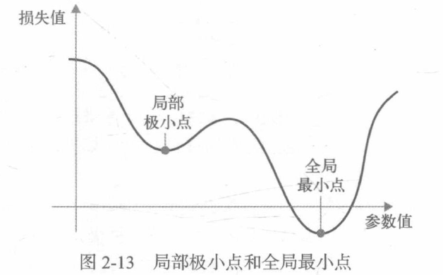
As shown in the figure, there is a local minimum point near a parameter value: near this point, moving left and right will increase the loss value. If the SGD of primary school learning rate is used for optimization, the optimization process may fall into a local minimum point, resulting in the inability to find the global minimum point. This problem can be avoided by using the momentum method.

past_velocity = 0
momentum = 0.1
while loss > 0.01:
    w, loss, gradient = get_current_parameters()
    velocity = past_velocity * momentum - learning_rate * gradient
    w = w + momentum * veloctiy - learning_rate * gradient
    past_velocity = velocity
    update_parameter(w)

2.4.4 chain derivation: back propagation algorithm

Applying the chain rule to the calculation of gradient value of neural network, the obtained algorithm is called back propagation, sometimes also called trans differentiation. Back propagation starts from the final loss value and acts in reverse from the top layer to the bottom layer. The contribution of each parameter to the loss value is calculated by using the chain rule.

Now and in the next few years, people will use modern frameworks that can carry out symbolic differentiation to realize neural networks, such as TensorFlow, that is, given an operation chain and the derivative of each operation is known, these frameworks can use the chain rule to calculate the gradient function of the operation chain and map the network parameter values into gradient values. For such a function, back propagation is simplified to calling the gradient function. Due to the emergence of symbolic differentiation, you do not need to manually implement the back-propagation algorithm.

2.5 review the first example

from keras.datasets import mnist
from keras import models
from keras import layers
import matplotlib.pyplot as plt

(train_images, train_labels), (test_images, test_labels) = mnist.load_data()

train_images = train_images.reshape((60000, 28 * 28))
train_images = train_images.astype('float32') / 255

test_images = test_images.reshape((10000, 28 * 28))
test_images = test_images.astype('float32') / 255

network = models.Sequential()
network.add(layers.Dense(512, activation='relu', input_shape=(28 * 28)))
network.add(layers.Dense(10, activation='softmax'))
network.compile(optimizer='rmsprop',
                loss = 'categorical_crossentropy',
                metrics=['accuracy'])
network.fit(train_images, train_labels, epochs=5, batch_size=128)

The network starts to iterate on the training data, with a total of 5 iterations (one iteration on all training data is called one round). In each iteration, the network calculates the gradient of batch loss relative to the weight and updates the weight accordingly. After five rounds, the network has 2345 gradient updates, and the network loss value will become small enough to enable the network to classify handwritten digits with high accuracy.

Summary of this chapter

1. Learning refers to finding a set of model parameters to minimize the loss function on a given training data sample and the corresponding target value.

2. Learning process: randomly select the batch containing data samples and their target values, calculate the gradient of batch loss to network parameters, and then move the network parameters slightly along the opposite direction of the gradient (the moving distance is specified by the learning rate).

3. The whole learning process can be realized because the neural network is a series of differentiable tensor operations. Therefore, the chain rule of derivation can be used to obtain the gradient function, which maps the current parameters and current data into a gradient value in batch.

4. Before inputting data into the network, you need to define the loss and optimizer.

5. Loss is the amount that needs to be minimized during training, so it should be able to measure whether the current task has been successfully solved.

6. The optimizer is a specific way to update parameters using loss gradient, such as RMSProp optimizer, random gradient descent with momentum (SGD), etc.

Topics: Python neural networks Deep Learning

Programmer Think