5.3 using pre trained convolutional neural networks
Pre trained network:
- It has been used in large data sets (usually large-scale image classification tasks) Training Practice good , protect Save good of network Collaterals \color{red} trained and preserved network Trained and preserved network.
- Pre training network learn reach of special sign of empty between layer second junction structure \color{red} learns the spatial hierarchy of features The spatial hierarchy of the learned features can be effectively used as a general model of the visual world, which has a wide range of problems can shift plant nature \color{red} portability Portability.
- Due to the pre training network, deep learning yes Small number according to ask topic wrong often have effect \color{red} is very effective for small data problems It is very effective for small data problems.
There are two ways to use the pre training network: special sign carry take ( f e a t u r e e x t r a c t i o n ) \color{red} feature extraction Feature extraction and tiny transfer model type ( f i n e − t u n i n g ) \color{red} fine tuning model fine tune the model.
5.3.1 feature extraction
-
definition:
special sign carry take yes send use of front network Collaterals learn reach of surface show come from new kind book in carry take Out have interest of special sign . \color{red} feature extraction uses the representations learned from the network to extract interesting features from new samples. Feature extraction is to extract interesting features from new samples using the representations learned from the network. -
volume product base \color{red} convolution basis Convolution basis:
- The convolutional neural network for image classification consists of two parts: the first is a series of pooling layers and convolution layers, and the last is a dense connection classifier. The first part is called model volume product base ( c o n v o l u t i o n a l b a s e ) \color{red} convolutional base Convolutional base.
- Feature extraction is to take out the convolution basis of the previously trained network, run new data on it, and then
stay
transport
Out
upper
noodles
Training
Practice
one
individual
new
of
branch
class
implement
\color{red} trains a new classifier on the output
Train a new classifier on the output.
- Why not use dense layers: the representation of dense connected layers no longer contains the objects in the input image position Set letter interest \color{red} location information Location information. The dense connection layer discards the concept of space, and the object position information is still described by the convolution characteristic graph.
- Extracted from a convolution layer
surface
show
of
through
use
nature
\Generality of color{red} representation
The commonality (and reusability) of the representation depends on
Should
layer
stay
model
type
in
of
deep
degree
\color{red} the depth of the layer in the model
The depth of the layer in the model.
In the model, the layer closer to the bottom extracts local and highly general feature images (such as visual edges, colors and textures), while the layer closer to the top extracts more abstract concepts (such as "cat ears" or "dog eyes").
- If your new data set is very different from the data set trained by the original model, it is best to use only the first few layers of the model for feature extraction, rather than the whole convolution basis.
- Common models are built into Keras. You can get it from Keras Import in the applications module.
-
VGG16 model
from tensorflow.keras.applications import VGG16
conv_base = VGG16(weights='imagenet',
				  include_top=False,
				  input_shape=(150, 150, 3))
Here, three parameters are passed into the constructor.
- weights specifies the weight checkpoint for model initialization.
- include_top specifies whether the model finally contains a dense join classifier. By default, this dense connection classifier corresponds to 1000 categories of ImageNet. Because we intend to use our own dense join classifier (only two categories: cat and dog), we don't need to include it.
- input_shape is the shape of the image tensor input into the network. This parameter is completely optional. If this parameter is not passed in, the network can handle any shape of input.
conv_base.summary()
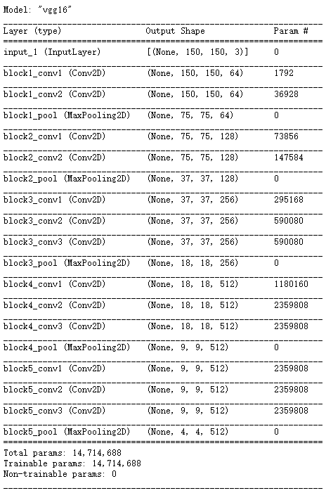
The final feature graph shape is (4, 4, 512). We will add a dense connection classifier to this feature. There are two options for the next step.
- Fast feature extraction without data enhancement.
This method has high speed and low computational cost, because it only needs to run the convolution basis once for each input image, and the convolution basis is the most expensive in the current process. - Feature extraction using data enhancement
Add a sense layer at the top to extend the existing model (i.e. conv_base) and run the whole model end-to-end on the input data.
5.3.1.1. Fast feature extraction without data enhancement
First, run the ImageDataGenerator instance to extract the image and its tags into a Numpy array. Call conv_base model is used to extract features from these images. Code of the first method: protect Save you of number according to stay \color{red} save your data in Save your data in conv_ Output in base, however after take this some transport Out do by transport enter use to new model type \color{red} then uses these outputs as input for the new model These outputs are then used as inputs for the new model.
-
Feature extraction using pre trained convolution basis
import os
import numpy as np
from tensorflow.keras.preprocessing.image import ImageDataGenerator

base_dir = 'C:\\Users\\Administrator\\deep-learning-with-python-notebooks-master\\cats_and_dogs_small'
train_dir = os.path.join(base_dir, 'train')
validation_dir = os.path.join(base_dir, 'validation')
test_dir = os.path.join(base_dir, 'test')

datagen = ImageDataGenerator(rescale=1./255)
batch_size = 20

def extract_features(directory, sample_count):
	features = np.zeros(shape=(sample_count, 4, 4, 512))
	labels = np.zeros(shape=(sample_count))
	generator = datagen.flow_from_directory(
		directory,
		target_size=(150, 150),
		batch_size=batch_size,
		class_mode='binary')
	i = 0
	for inputs_batch, labels_batch in generator:
		features_batch = conv_base.predict(inputs_batch)
		features[i * batch_size : (i + 1) * batch_size] = features_batch
		labels[i * batch_size : (i + 1) * batch_size] = labels_batch
		i += 1
		if i * batch_size >= sample_count:
			break
	# Note that these generators constantly generate data in the loop,
	# So you have to end the loop after reading all the images
	return features, labels

train_features, train_labels = extract_features(train_dir, 4000)
validation_features, validation_labels = extract_features(validation_dir, 2000)
test_features, test_labels = extract_features(test_dir, 2000)

# The extracted feature shapes are (samples, 4, 4, 512). We need to input it into the dense connection classifier,
# So you must first flatten the shape to (samples, 8192)
train_features = np.reshape(train_features, (4000, 4 * 4 * 512))
validation_features = np.reshape(validation_features, (2000, 4 * 4 * 512))
test_features = np.reshape(test_features, (2000, 4 * 4 * 512))
-
Define and train dense join classifiers
You need to use dropout regularization and train the classifier on the just saved data and tags.from tensorflow.keras import models from tensorflow.keras import layers from tensorflow.keras import optimizers model = models.Sequential() model.add(layers.Dense(256, activation='relu', input_dim=4 * 4 * 512)) model.add(layers.Dropout(0.5)) model.add(layers.Dense(1, activation='sigmoid')) model.compile(optimizer=optimizers.RMSprop(lr=2e-5), loss='binary_crossentropy', metrics=['acc']) history = model.fit(train_features, train_labels, epochs=30, batch_size=20, validation_data=(validation_features, validation_labels))
-
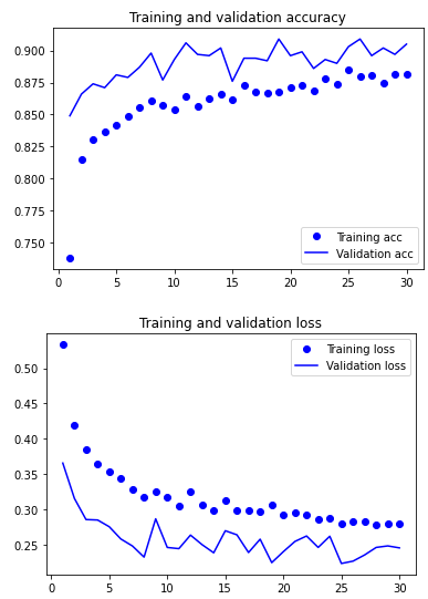
Draw results
import matplotlib.pyplot as plt

acc = history.history['acc']
val_acc = history.history['val_acc']
loss = history.history['loss']
val_loss = history.history['val_loss']

epochs = range(1, len(acc) + 1)

plt.plot(epochs, acc, 'bo', label='Training acc')
plt.plot(epochs, val_acc, 'b', label='Validation acc')
plt.title('Training and validation accuracy')
plt.legend()

plt.figure()

plt.plot(epochs, loss, 'bo', label='Training loss')
plt.plot(epochs, val_loss, 'b', label='Validation loss')
plt.title('Training and validation loss')
plt.legend()
plt.show()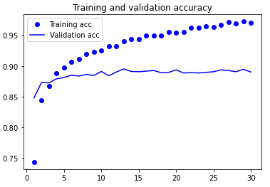

Although the dropout ratio is quite large, the model is over fitted almost from the beginning. that is because book square method no have send use number according to increase strong \color{red} This method does not use data enhancement This method does not use data enhancement, but number according to increase strong yes Guard against stop Small type chart image number according to collection of too Draft close wrong often heavy want \color{red} data enhancement is very important to prevent over fitting of small image data sets Data enhancement is very important to prevent over fitting of small image data sets.
5.3.1.2. Feature extraction using data enhancement
It is slower and more computationally expensive, but data enhancement can be used during training. This method is: expand exhibition \color{red} extension Extended conv_base model, however after stay transport enter number according to upper end reach end land transport that 's ok model type \color{red} then run the model end-to-end on the input data Then run the model end-to-end on the input data.
The calculation cost of this method is very high, and it can only be tried when there is a GPU. It is absolutely difficult to run on the CPU. If you can't run code on the GPU, use the first method.
- A dense connection classifier is added to the convolution basis
from tensorflow.keras import models
from tensorflow.keras import layers

model = models.Sequential()
model.add(conv_base)
model.add(layers.Flatten())
model.add(layers.Dense(256, activation='relu'))
model.add(layers.Dense(1, activation='sigmoid'))
model.summary()
- The convolution basis of VGG16 has 14714688 parameters, very many. The classifier added to it has 2 million parameters.
- The convolution basis must be "frozen" before compiling and training the model. freeze junction \color{red} freeze freeze one or more layers means to keep their weights unchanged during training. If this is not done, the previously learned representation of the convolution basis will be modified during the training process. Because the density layer added on it is randomly initialized, very large weight updates will spread in the network, causing great damage to the previously learned representation.
- Freezing model
In Keras, freeze junction network Collaterals of square method yes take his t r a i n a b l e genus nature set up by F a l s e \color{red} the way to freeze the network is to set its trainable property to False The way to freeze a network is to set its trainable property to False.
After setting, only the weights of the two density layers added will be trained. There are four weight tensors in total, two in each layer (sovereign weight matrix and bias vector).>>> print('This is the number of trainable weights ' 'before freezing the conv base:', len(model.trainable_weights)) This is the number of trainable weights before freezing the conv base: 30 >>> conv_base.trainable = False >>> print('This is the number of trainable weights ' 'after freezing the conv base:', len(model.trainable_weights)) This is the number of trainable weights after freezing the conv base: 4If the trainable attribute of the weight is modified after compilation, the model should be recompiled, otherwise these modifications will be ignored.
- End to end training model using frozen convolution base
from tensorflow.keras.preprocessing.image import ImageDataGenerator
from tensorflow.keras import optimizers
train_datagen = ImageDataGenerator(
	rescale=1./255,
	rotation_range=40,
	width_shift_range=0.2,
	height_shift_range=0.2,
	shear_range=0.2,
	zoom_range=0.2,
	horizontal_flip=True,
	fill_mode='nearest')

# Note that validation data cannot be enhanced
test_datagen = ImageDataGenerator(rescale=1./255)

train_generator = train_datagen.flow_from_directory(
	train_dir,#Target directory
	target_size=(150, 150),# Resize all images to 150 × one hundred and fifty
	batch_size=20,
	class_mode='binary')
	#Because binary is used_ Crossintropy is lost, so you need to use binary tags

validation_generator = test_datagen.flow_from_directory(
	validation_dir,
	target_size=(150, 150),
	batch_size=20,
	class_mode='binary')
model.compile(loss='binary_crossentropy',
	optimizer=optimizers.RMSprop(lr=2e-5),
	metrics=['acc'])
history = model.fit_generator(
	train_generator,
	steps_per_epoch=200,#The data is 4000
	epochs=30,
	validation_data=validation_generator,
	validation_steps=50)
5.3.2 fine tuning model
-
model type tiny transfer ( f i n e − t u n i n g ) \color{red} model fine tuning fine tuning and feature extraction mutual by repair charge \color{red} complements each other They complement each other.
-
tiny transfer model type set righteousness \color{red} fine tune model definition Fine tune model definition:
For the frozen model base used for feature extraction, fine tuning refers to top Department of A few layer " solution freeze " \Several layers of "thaw" at the top of color{red} The top layers are "thawed" and will solution freeze of A few layer and new increase plus of Department branch Couplet close Training Practice \color{red} thawed layers and newly added parts of joint training Thawed layers and newly added parts of joint training. For this example, fine tuning is to tune the last part of the original and the new part.- freeze junction V G G 16 of volume product base yes by Yes can enough stay upper noodles Training Practice one individual along with machine first beginning turn of branch class implement . \color{red} the convolution basis of VGG16 is frozen so that a randomly initialized classifier can be trained on it. The convolution basis of VGG16 is frozen so that a randomly initialized classifier can be trained on it.
-
only
have
upper
noodles
of
branch
class
implement
already
through
Training
Practice
good
Yes
,
just
can
tiny
transfer
volume
product
base
of
top
Department
A few
layer
.
\color{red} only after the above classifier has been trained can the top layers of convolution basis be fine tuned.
Only when the above classifier has been trained can the top layers of convolution basis be fine tuned.

-
To fine tune a network
- stay already through Training Practice good of base network Collaterals ( b a s e n e t w o r k ) upper add plus since set righteousness network Collaterals \color{red} add a custom network to the trained base network Add a custom network to the trained base network.
- freeze junction base network Collaterals \color{red} freeze base network Freeze the base network.
- Training Practice place add plus of Department branch \Part added by color{red} training The part added to the training.
- solution freeze base network Collaterals of one some layer \color{red} thaws some layers of the base network Thaw some layers of the base network.
- Couplet close Training Practice solution freeze of this some layer and add plus of Department branch \color{red} joint training thawed these layers and added parts Joint training thawed these layers and added parts.
The first three steps are feature extraction.
-
Why more by top layer do tiny transfer \color{blue} is more fine tuned by the top layer More fine-tuning on the top?
- Convolution basis more by bottom Department of layer Compile code of yes more plus through use of can complex use special sign \color{red} the layer at the bottom encodes more general reusable features The layer closer to the bottom encodes more general reusable features, while the layer closer to the top encodes more specialized features.
- Training Practice of ginseng number More many , too Draft close of wind Risk More large \The more parameters of color{red} training, the greater the risk of over fitting The more training parameters, the greater the risk of over fitting.
-
Freeze all layers up to a layer
conv_base.trainable = True

set_trainable = False
for layer in conv_base.layers:
	if layer.name == 'block5_conv1':
		set_trainable = True
	if set_trainable:
		layer.trainable = True
	else:
		layer.trainable = False

-
Fine tuning model
model.compile(loss='binary_crossentropy',
	optimizer=optimizers.RMSprop(lr=1e-5),
	metrics=['acc'])
history = model.fit_generator(
	train_generator,
	steps_per_epoch=200,
	epochs=100,
	validation_data=validation_generator,
	validation_steps=50)
-
Smoothes the curve
import matplotlib.pyplot as plt
def smooth_curve(points, factor=0.8):
	smoothed_points = []
	for point in points:
		if smoothed_points:
			previous = smoothed_points[-1]
			smoothed_points.append(previous * factor + point * (1 - factor))
		else:
			smoothed_points.append(point)
	return smoothed_points
plt.plot(epochs,
	smooth_curve(acc), 'bo', label='Smoothed training acc')
plt.plot(epochs,
	smooth_curve(val_acc), 'b', label='Smoothed validation acc')
plt.title('Training and validation accuracy')
plt.legend()
plt.figure()
plt.plot(epochs,
	smooth_curve(loss), 'bo', label='Smoothed training loss')
plt.plot(epochs,
	smooth_curve(val_loss), 'b', label='Smoothed validation loss')
plt.title('Training and validation loss')
plt.legend()
plt.show()
Epoch 97/100 200/200 [==============================] - 224s 1s/step - loss: 0.0158 - acc: 0.9950 - val_loss: 0.3688 - val_acc: 0.9450 Epoch 98/100 200/200 [==============================] - 223s 1s/step - loss: 0.0153 - acc: 0.9945 - val_loss: 0.4035 - val_acc: 0.9410 Epoch 99/100 200/200 [==============================] - 223s 1s/step - loss: 0.0260 - acc: 0.9901 - val_loss: 0.3588 - val_acc: 0.9440 Epoch 100/100 200/200 [==============================] - 223s 1s/step - loss: 0.0155 - acc: 0.9946 - val_loss: 0.4835 - val_acc: 0.9410
The accuracy is improved to 94%, and the loss curve does not change much.
From the loss curve, there is no real improvement (actually getting worse) compared with before. If the loss is not reduced, how can the accuracy remain stable or improved? The answer is simple: the figure shows the average point wise loss, but shadow ring essence degree of yes damage lose value of branch cloth \color{red} what affects the accuracy is the distribution of loss values It is the distribution of loss values rather than the average value that affects the accuracy, because the accuracy is the binary threshold of the category probability predicted by the model. Even if it cannot be seen from the average loss, the model may still be improving.
5.3.2.1 final evaluation of this model
test_generator = test_datagen.flow_from_directory(
	test_dir,
	target_size=(150, 150),
	batch_size=20,
	class_mode='binary')

test_loss, test_acc = model.evaluate_generator(test_generator, steps=50)
print('test acc:', test_acc)
5.3.3 summary
Image classification problem, especially for Small type number according to collection \color{red} small dataset Small datasets:
- volume product god through network Collaterals yes use to meter count machine regard sleep let Affairs of most good machine implement learn Learn model type \color{red} convolutional neural network is the best machine learning model for computer vision tasks Convolutional neural network is the best machine learning model for computer vision tasks. A convolutional neural network can be trained from scratch even on a very small data set, and the results are good.
- stay Small type number according to collection upper of main want ask topic yes too Draft close \The main problem of color{red} on small data sets is over fitting The main problem on small data sets is over fitting. When processing image data, number according to increase strong \color{red} data enhancement Data enhancement is a powerful method to reduce over fitting.
- utilize special sign carry take \color{red} feature extraction Feature extraction can easily integrate the existing convolutional neural network complex use \color{red} reuse Reuse in new data sets. This is a valuable method for small image data sets.
- As a supplement to feature extraction, you can also use tiny transfer \color{red} fine tuning Fine tune and apply some data representations learned before the existing model to new problems. This method can further improve the performance of the model.
Complete code
## Data preparation
import os, shutil
# The path to the original dataset decompression directory
original_dataset_dir = 'C:\\Users\\Administrator\\Python_learning\\kaggle_original_data'
# Directory to save smaller datasets
base_dir = 'C:\\Users\\Administrator\\Python_learning\\cats_and_dogs_small'
os.mkdir(base_dir)

# Corresponding to the directory of divided training, verification and test respectively
train_dir = os.path.join(base_dir, 'train')
os.mkdir(train_dir)
validation_dir = os.path.join(base_dir, 'validation')
os.mkdir(validation_dir)
test_dir = os.path.join(base_dir, 'test')
os.mkdir(test_dir)

# Cat training image directory
train_cats_dir = os.path.join(train_dir, 'cats')
os.mkdir(train_cats_dir)
# Dog training image directory
train_dogs_dir = os.path.join(train_dir, 'dogs')
os.mkdir(train_dogs_dir)
# Cat authentication image directory
validation_cats_dir = os.path.join(validation_dir, 'cats')
os.mkdir(validation_cats_dir)
# Dog authentication image directory
validation_dogs_dir = os.path.join(validation_dir, 'dogs')
os.mkdir(validation_dogs_dir)
# Cat test image directory
test_cats_dir = os.path.join(test_dir, 'cats')
os.mkdir(test_cats_dir)
# Dog test image directory
test_dogs_dir = os.path.join(test_dir, 'dogs')
os.mkdir(test_dogs_dir)

# Copy the first 2000 cat images to the train_cats_dir
fnames = ['cat.{}.jpg'.format(i) for i in range(2000)]
for fname in fnames:
    src = os.path.join(original_dataset_dir, fname)
    dst = os.path.join(train_cats_dir, fname)
    shutil.copyfile(src, dst)
# Copy the next 1000 cat images to validation_cats_dir
fnames = ['cat.{}.jpg'.format(i) for i in range(2000, 3000)]
for fname in fnames:
    src = os.path.join(original_dataset_dir, fname)
    dst = os.path.join(validation_cats_dir, fname)
    shutil.copyfile(src, dst)
# Copy the next 1000 cat images to test_cats_dir
fnames = ['cat.{}.jpg'.format(i) for i in range(3000, 4000)]
for fname in fnames:
    src = os.path.join(original_dataset_dir, fname)
    dst = os.path.join(test_cats_dir, fname)
    shutil.copyfile(src, dst)

# Copy the first 2000 dog images to the train_dogs_dir
fnames = ['dog.{}.jpg'.format(i) for i in range(2000)]
for fname in fnames:
    src = os.path.join(original_dataset_dir, fname)
    dst = os.path.join(train_dogs_dir, fname)
    shutil.copyfile(src, dst)
# Copy the next 1000 dog images to validation_dogs_dir
fnames = ['dog.{}.jpg'.format(i) for i in range(2000, 3000)]
for fname in fnames:
    src = os.path.join(original_dataset_dir, fname)
    dst = os.path.join(validation_dogs_dir, fname)
    shutil.copyfile(src, dst)
# Copy the next 1000 dog images to test_dogs_dir
fnames = ['dog.{}.jpg'.format(i) for i in range(3000, 3000)]
for fname in fnames:
    src = os.path.join(original_dataset_dir, fname)
    dst = os.path.join(test_dogs_dir, fname)
    shutil.copyfile(src, dst)

## Data preprocessing, using data enhancement
train_datagen = ImageDataGenerator(
	rescale=1./255,
	rotation_range=40,
	width_shift_range=0.2,
	height_shift_range=0.2,
	shear_range=0.2,
	zoom_range=0.2,
	horizontal_flip=True,)
# Note that validation data cannot be enhanced
test_datagen = ImageDataGenerator(rescale=1./255)
train_generator = train_datagen.flow_from_directory(
		train_dir,               # Target directory
		target_size=(150, 150),  # Resize all images to 150 × one hundred and fifty
		batch_size=20,
		# It's 32 in the book, but 32*200(steps_per_epoch) is greater than 4000. An error will be reported during operation, so it's changed to 20
		class_mode='binary')
# Because binary is used_ Crossintropy is lost, so you need to use binary tags

validation_generator = test_datagen.flow_from_directory(
		validation_dir,
		target_size=(150, 150),
		batch_size=20, # It's 32 in the book, but 32*200(steps_per_epoch) is greater than 4000. An error will be reported during operation, so it's changed to 20
		class_mode='binary')

## Call VGG16
from tensorflow.keras.applications import VGG16
conv_base = VGG16(weights='imagenet',
				  include_top=False,
				  input_shape=(150, 150, 3))

## Feature extraction using data enhancement
# A dense connection classifier is added to the convolution basis
from tensorflow.keras import models
from tensorflow.keras import layers

model = models.Sequential()
model.add(conv_base)
model.add(layers.Flatten())
model.add(layers.Dense(256, activation='relu'))
model.add(layers.Dense(1, activation='sigmoid'))

## Fine tuning model
conv_base.trainable = True

set_trainable = False
for layer in conv_base.layers:
	if layer.name == 'block5_conv1':
		set_trainable = True
	if set_trainable:
		layer.trainable = True
	else:
		layer.trainable = False

# Training model
model.compile(loss='binary_crossentropy',
	optimizer=optimizers.RMSprop(lr=1e-5),
	metrics=['acc'])
history = model.fit_generator(
	train_generator,
	steps_per_epoch=200,
	epochs=100,
	validation_data=validation_generator,
	validation_steps=50)

## Draw smooth curve
def smooth_curve(points, factor=0.8):
	smoothed_points = []
	for point in points:
		if smoothed_points:
			previous = smoothed_points[-1]
			smoothed_points.append(previous * factor + point * (1 - factor))
		else:
			smoothed_points.append(point)
	return smoothed_points
plt.plot(epochs,
	smooth_curve(acc), 'bo', label='Smoothed training acc')
plt.plot(epochs,
	smooth_curve(val_acc), 'b', label='Smoothed validation acc')
plt.title('Training and validation accuracy')
plt.legend()
plt.figure()
plt.plot(epochs,
	smooth_curve(loss), 'bo', label='Smoothed training loss')
plt.plot(epochs,
	smooth_curve(val_loss), 'b', label='Smoothed validation loss')
plt.title('Training and validation loss')
plt.legend()
plt.show()

## Evaluating models on test sets
test_generator = test_datagen.flow_from_directory(
	test_dir,
	target_size=(150, 150),
	batch_size=20,
	class_mode='binary')

test_loss, test_acc = model.evaluate_generator(test_generator, steps=50)
print('test acc:', test_acc)