Introduction to deep learning: Theory and Implementation Based on Python reading notes: Chapter 6 learning related skills

The learning purpose of neural network is to find the parameters that make the value of loss function as small as possible. This is the problem of finding the optimal parameters. The process of solving this problem is called optimization.

In order to find the optimal parameter, we take the gradient (derivative) of the parameter as the clue. Using the gradient of parameters, update the parameters along the gradient direction, and repeat this step many times, so as to gradually approach the optimal parameters. This process is called random descent gradient algorithm, or SGD for short. In this chapter, we will point out the shortcomings of SGD and introduce other optimization methods other than SGD.

6.1.1 explorer's story

Although the Explorer can't see the surrounding situation, he can know the slope of the current position (feel the inclination of the ground through the soles of his feet). Therefore, SGD's strategy is to move towards the direction with the largest slope at the current location. Brave explorers may think that as long as they repeat this strategy, they can reach the "deepest place" one day.

6.1.2 SGD

SGD can be written into the following formula with mathematical formula:

class SGD:
    def __init__(self, lr=0.01):
        self.lr = lr
    
    def update(self, params, grads):
        for key in params.keys():
            params[key] -= self.lr * grads[key]

Using this SGD class, the parameters of the neural network can be updated as follows (the following code is a pseudo code that cannot be actually run):

network = TwoLayerNet(...)
optimizer = SGD()

for i in range(10000):
    ...
    x_batch, t_batch = get_mini_batch(...) # mini_batch
    grads = network.gradient(x_batch, t_batch)
    params = network.params
    optimizer.update(params, grads)

Many deep learning frameworks implement various optimization methods, and provide structures that can simply switch these methods, from which users can choose the optimization methods they want to use.

6.1.3 disadvantages of SGD

Although SGD is simple and easy to implement, it may not be efficient in solving some problems.

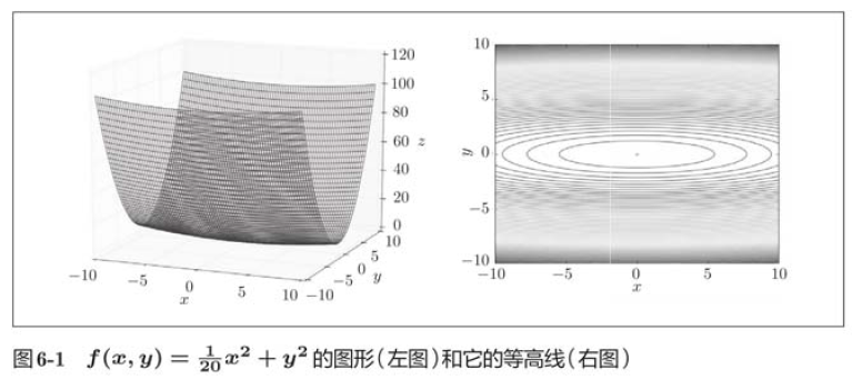
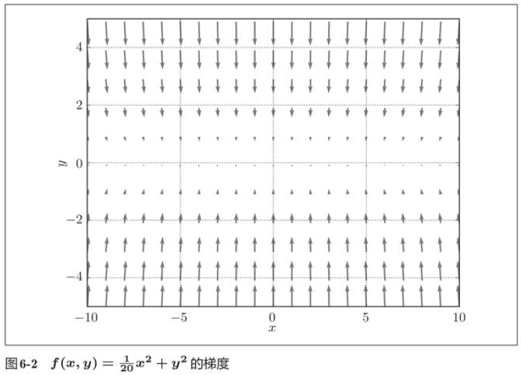
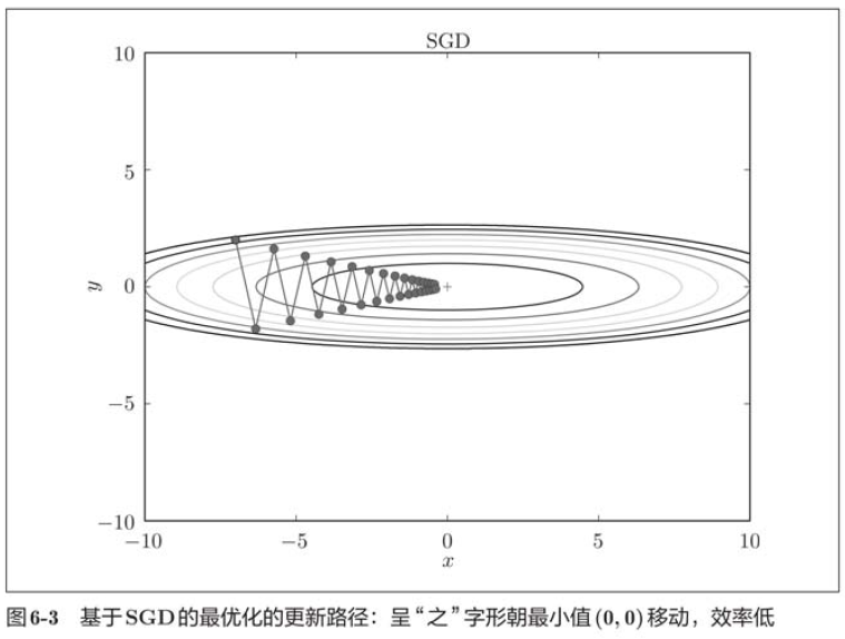
In the figure above, SGD moves in a zigzag shape, which is a rather inefficient path. In other words, the disadvantage of SGD is that if the shape of the function is non-uniform, such as extending, the search path will be very inefficient. Therefore, we need a smarter method than SGD simply moving in the direction of gradient. The root cause of SGD inefficiency is that the direction of gradient does not point to the direction of minimum value.

In order to correct the shortcomings of SGD, we will introduce three methods: Momentum, AdaGrad and Adam to replace SGD.

6.1.4 Momentum

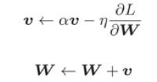
As shown in the figure above, the Momentum method feels like a small ball rolling on the ground.

import numpy as np


class Momentum:
    def __init__(self, lr=0.01, momentum=0.9):
        self.lr = lr
        self.momentum = momentum
        self.v = None
        
    def update(self, params, grads):
        if self.v is None:
            self.v = {}
            for key, val in params.items():
                self.v[key] = np.zeros_like(val)
                
        for key in params.keys():
            self.v[key] = self.momentum * self.v[key] - self.lr*grads[key]
            params[key] += self.v[key]

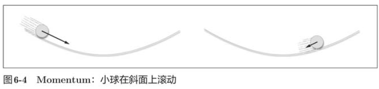
In the image above, the update path is like a ball rolling in a bowl. Compared with SGD, we found that the "degree" of zigzag was reduced. This is because although the force in the x-axis direction is very small, it is always in the same direction, so there will be a certain acceleration in the same direction. On the contrary, although the force in the y-axis direction is large, they will offset each other because they are interactively subjected to the forces in the positive and negative directions, so the velocity in the y-axis direction is unstable. Therefore, compared with the case of SGD, it can approach towards the x-axis faster and weaken the variation degree of "zigzag".

6.1.5 AdaGrad

In the learning of neural network, the learning rate (recorded in the mathematical formula as)The value of is important. If the learning rate is too small, it will lead to excessive time spent on learning; Conversely, if the learning rate is too high, it will lead to learning divergence and can not be carried out correctly.

Among the effective skills about learning rate, there is a method called learning rate attenuation, that is, the learning rate decreases gradually with the progress of learning. In fact, the method of "learning more" at first and then "learning less" gradually is often used in the learning of neural networks.

The idea of gradually reducing the learning rate is equivalent to reducing the learning rate value of "all" parameters. AdaGrad further developed this idea and gave "customized" values to "one by one" parameters.

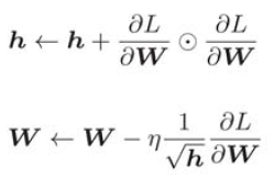
AdaGrad will adjust the learning rate appropriately for each element of the parameter and learn at the same time.

AdaGrad records the sum of squares of all gradients in the past. Therefore, the deeper the learning, the smaller the range of updating. In fact, if you study endlessly, the update amount will become 0 and will not be updated at all. In order to improve this problem, RMSProp method can be used. This method does not add all the gradients in the past equally, but gradually forgets the gradients in the past, and more reflects the information of the new gradient when doing addition operation. Professionally speaking, this operation is called "exponential moving average", which exponentially reduces the scale of the past gradient.

import numpy as np


class AdaGrad:
    def __init__(self, lr=0.01):
        self.lr = lr
        self.h = None
        
    def update(self, params, grads):
        if self.h is None:
            self.h = {}
            for key, val in params.items():
                self.h[key] = np.zeros_like(val)
        
        for key in params.keys():
            self.h[key] += grads[key] * grads[key]
            params[key] -= self.lr * grads[key] / (np.sqrt(self.h[key]) + 1e-7)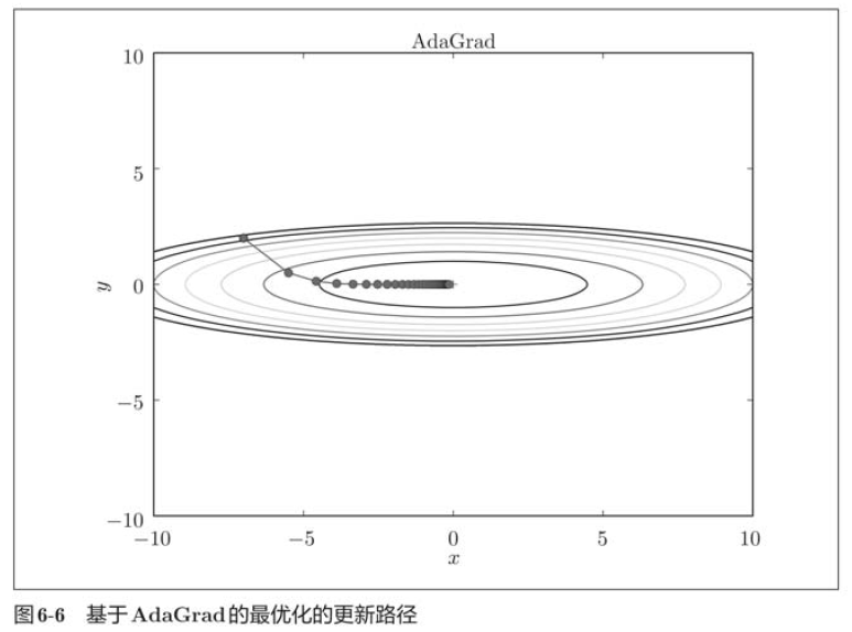

It can be seen from the results above that the value of the function moves towards the minimum value efficiently. Due to the large gradient in the y-axis direction, it changes greatly at the beginning, but it will be adjusted proportionally according to this large change to reduce the pace of update. Therefore, the update degree in the y-axis direction is weakened, and the change degree of zigzag is attenuated.

6.1.6 Adam

Momentum moves according to the physical rules of the ball rolling in the bowl, and AdaGrad appropriately adjusts the update pace for each element of the parameter. What will happen if these two methods are combined? This is the basic idea of Adam's method.

import numpy as np


class Adam:
    def __init__(self, lr=0.01, beta1=0.9, beta2=0.999):
        self.lr = lr
        self.beta1 = beta1
        self.beta2 = beta2
        self.iter = 0
        self.m = None
        self.v = None
        
    def update(self, params, grads):
        if self.m is None:
            self.m, self.v = {}, {}
            for key, val in params.items():
                self.m[key] = np.zeros_like(val)
                self.v[key] = np.zeros_like(val)
        
        self.iter += 1
        lr_t = self.lr * np.sqrt(1.0 - self.beta2**self.iter) / (1.0 - self.beta1**self.iter)
        
        for key in params.keys():
            self.m[key] += (1 - self.beta1) * (grads[key] - self.m[key])
            self.v[key] += (1 - self.beta2) * (grads[key]**2 - self.v[key])
            
            params[key] -= lr_t * self.m[key] / (np.sqrt(self.v[key]) + 1e-7)

In the above figure, the update process based on Adam is like a small ball rolling in a bowl. Although Momentum also moves similarly, in contrast, the shaking degree of Adam's small ball from left to right is reduced, which is due to the appropriate adjustment of the update degree of learning.

6.1.7 which update method to use

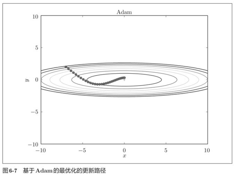
At present, there is no method that can perform well in all problems. These four methods have their own characteristics, and they all have problems they are good at solving and problems they are not good at solving.

6.1.8 comparison of update methods based on MNIST dataset

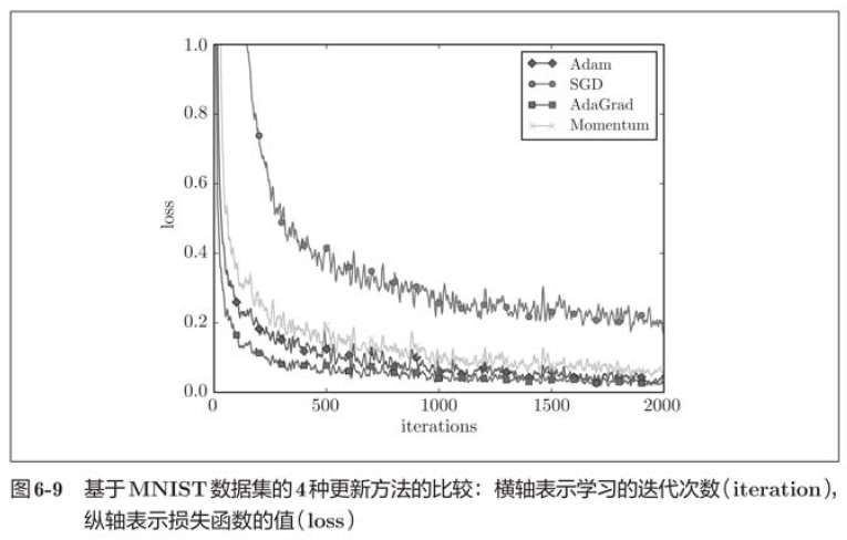Generally speaking, compared with SGD, the other three methods can learn faster, and some final recognition accuracy is also higher.

6.2 initial value of weight

6.2.1 can the initial value of weight be set to 0

Weight attenuation is a learning method aimed at reducing the value of weight parameters, which suppresses the occurrence of over fitting by reducing the value of weight parameters.

If you want to reduce the value of the weight, it is the right way to set the initial value to a smaller value at the beginning. What happens if we set the initial value of the weight to all 0 to reduce the value of the weight? In conclusion, setting the initial value of the weight to 0 is not a good idea. In fact, if the initial value of the weight is set to 0, it will not be able to learn correctly. In order to prevent "weight homogenization" (strictly speaking, to disintegrate the symmetrical structure of weight), the initial value must be randomly generated.

6.2.2 distribution of activation values of hidden layers

Let's do a simple experiment to observe how the initial value of weight affects the distribution of activation value of hidden layer. The experiment to be done here is to input randomly generated input data to a five layer neural network (the activation function uses sigmoid function), and draw the data distribution of activation values of each layer with histogram.

import numpy as np
import matplotlib.pyplot as plt


def sigmoid(x):
    return 1 / (1 + np.exp(-x))


def ReLU(x):
    return np.maximum(0, x)


def tanh(x):
    return np.tanh(x)


input_data = np.random.randn(1000, 100)
node_num = 100
hidden_layer_size = 5
activations = {}

x = input_data

for i in range(hidden_layer_size):
    if i != 0:
        x = activations[i-1]

    w = np.random.randn(node_num, node_num) * 1
    a = np.dot(x, w)
    z = sigmoid(a)
    activations[i] = z

for i, a in activations.items():
    plt.subplot(1, len(activations), i+1)
    plt.title(str(i+1) + '-layer')
    if i != 0:
        plt.yticks([], [])
    plt.hist(a.flatten(), 30, range=(0, 1))

plt.show()

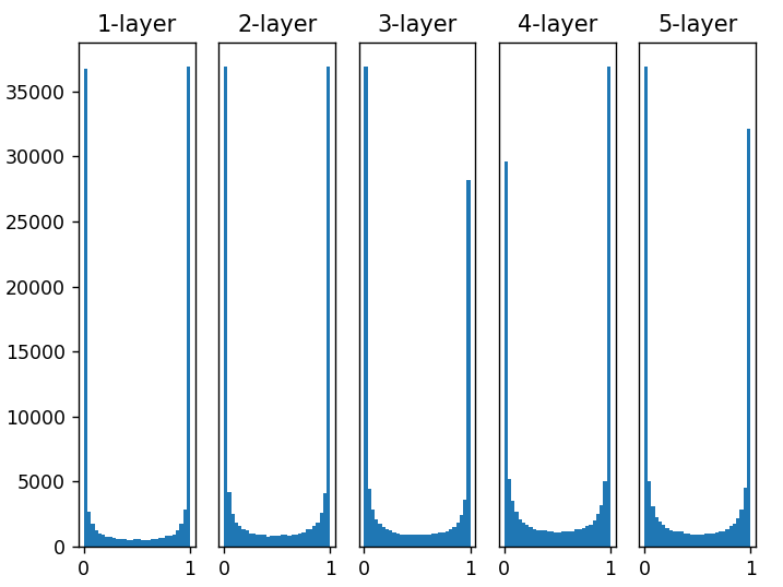
It can be seen from the above figure that the activation values of each layer are biased towards 0 and 1. The sigmoid function used here is an S-type function. As the output keeps approaching 0 (or 1), the value of its derivative gradually approaches 0. Therefore, the data distribution biased towards 0 and 1 will cause the value of the gradient in back propagation to become smaller and disappear. This problem is called gradient disappearance. In deep learning with deeper levels, the problem of gradient disappearance may be more serious.

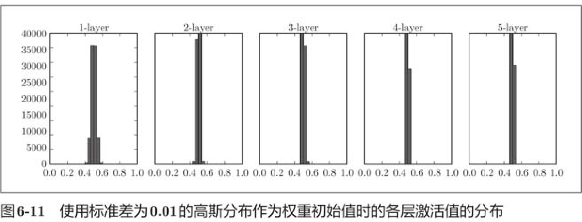
    # w = np.random.randn(node_num, node_num) * 1
    w = np.random.randn(node_num, node_num) * 0.01

The distribution of activation values in each layer requires an appropriate breadth, because neural networks can learn efficiently by transmitting diverse data between layers. Conversely, if biased data is transmitted, the gradient will disappear or the problem of "limited expressiveness" will appear, resulting in the failure of learning.

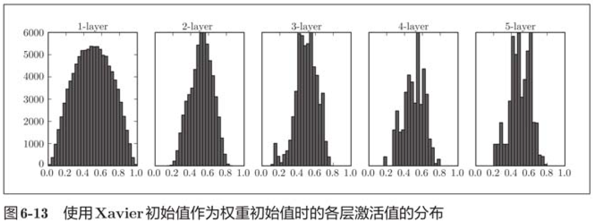It can be seen from the above figure that the more the back layer is, the more skewed the image becomes, but it presents a wider distribution than before. Because the data transmitted between layers has an appropriate breadth, the expressiveness of sigmoid function is not limited, and it is expected to learn efficiently.

6.2.3 initial weight value of relu

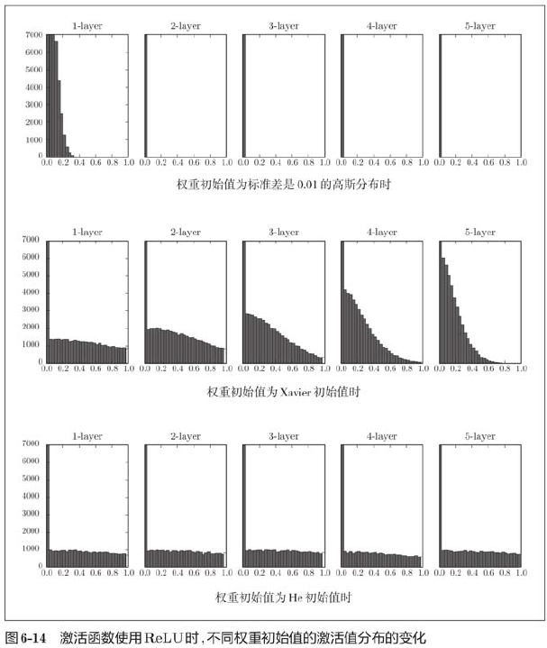
The experimental results show that when "std=0.01", the activation value of each layer is very small. The neural network transmits a very small value, indicating that the gradient of weight in reverse propagation is also very small, which is a very serious problem. In fact, there is little progress in learning.

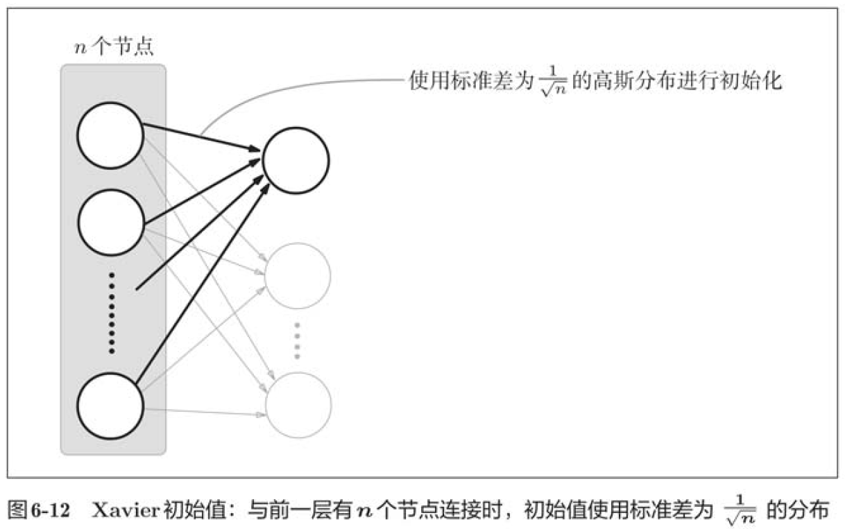
Next is the result when the initial value is Xavier initial value. In this case, as the layer deepens, the bias becomes larger. In fact, when the layer deepens, the bias of activation value becomes larger, and the gradient disappears during learning. When the initial value is He initial value, the distribution width in each layer is the same. Since the breadth of data can remain unchanged even if the layer is deepened, appropriate values will be passed during reverse propagation.

To sum up, when the activation function uses ReLU, the initial value of weight uses He initial value, and when the activation function is sigmoid or tanh S-curve function, the initial value uses Xavier initial value. This is current best practice.

6.2.4 comparison of initial weight values based on MNIST data set

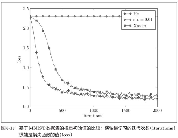
It can be seen from the above figure that learning is completely impossible when std=0.01, which is the same as the distribution of activation values just observed, because the value transmitted in the forward propagation is very small (data concentrated near 0). Therefore, the gradient obtained during reverse propagation is also very small, and the weight is hardly updated. On the contrary, when the weight initial value is Xavier initial value and He initial value, the learning goes well, and we find that the learning progress is faster when He initial value is used.

To sum up, the initial value of weight is very important in the learning of neural network. Many times, the setting of the initial value of weight is related to the success of neural network learning. The importance of weight initial value is easy to be ignored, and the beginning of anything (initial value) is always critical.

6.3 Batch Normalization

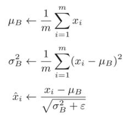
6.3.1 Batch Normalization algorithm

Batch Norm has the following advantages:

1. Learning can be carried out quickly (learning rate can be increased);

2. Less dependent on the initial value (less neurotic for the initial value);

3. Suppress over fitting (reduce the necessity of Dropout, etc.).

The idea of batch normal is to adjust the activation value distribution of each layer so that it has an appropriate breadth. Therefore, a layer that normalizes the data distribution, namely Batch Normalization layer (hereinafter referred to as batch normal layer), should be inserted into the neural network.

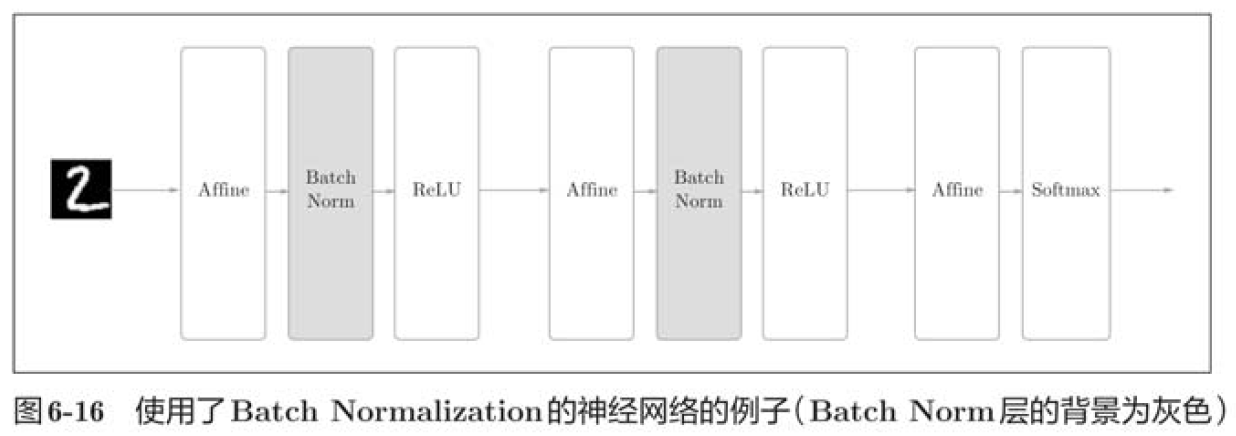
As the name suggests, Batch Norm is normalized by mini batch in the unit of mini batch during learning. Specifically, it is to normalize the data distribution with a mean of 0 and a variance of 1.

6.3.2 evaluation of batch normalization

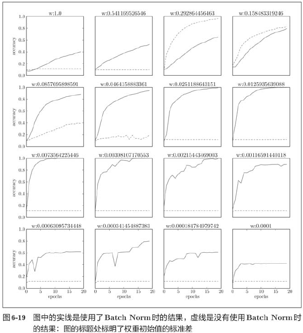
First, using the MNIST dataset, observe how the learning process changes with and without the Batch Norm layer.

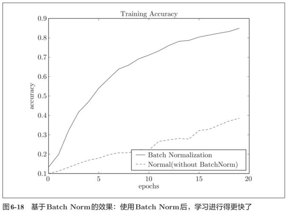We found that in almost all cases, learning proceeded faster when using Batch Norm. At the same time, it can also be found that in fact, without using Batch Norm, if you do not give a good initial value, the learning will be completely impossible.

To sum up, using Batch Norm can promote learning. Moreover, the initial value of the weight becomes robust ("robust to the initial value" means that it is less dependent on the initial value).

6.4 regularization

Over fitting is a very common problem in machine learning. Over fitting refers to the state that only the training data can be fitted, but other data not included in the training data can not be well fitted. Even if the training data is not included in the machine, it is hoped that the target recognition ability can be improved. We can make complex and expressive models, but accordingly, the technique of restraining over fitting is also very important.

6.4.1 over fitting

There are two main reasons for fitting.

1. The model has a large number of parameters and strong expressiveness;

2. Less training data.

Here, we deliberately meet these two conditions and create a fitting phenomenon.

import os
import sys

sys.path.append(os.pardir)  # Settings for importing files from the parent directory
import numpy as np
import matplotlib.pyplot as plt
from dataset.mnist import load_mnist
from common.multi_layer_net import MultiLayerNet
from common.optimizer import SGD

(x_train, t_train), (x_test, t_test) = load_mnist(normalize=True)

# In order to reproduce the over fitting, reduce the learning data
x_train = x_train[:300]
t_train = t_train[:300]

# Setting of weight decay=======================
#weight_decay_lambda = 0 # Without weight attenuation
weight_decay_lambda = 0.1
# ====================================================

network = MultiLayerNet(input_size=784, hidden_size_list=[100, 100, 100, 100, 100, 100], output_size=10,
                        weight_decay_lambda=weight_decay_lambda)
optimizer = SGD(lr=0.01)

max_epochs = 201
train_size = x_train.shape[0]
batch_size = 100

train_loss_list = []
train_acc_list = []
test_acc_list = []

iter_per_epoch = max(train_size / batch_size, 1)
epoch_cnt = 0

for i in range(1000000000):
    batch_mask = np.random.choice(train_size, batch_size)
    x_batch = x_train[batch_mask]
    t_batch = t_train[batch_mask]

    grads = network.gradient(x_batch, t_batch)
    optimizer.update(network.params, grads)

    if i % iter_per_epoch == 0:
        train_acc = network.accuracy(x_train, t_train)
        test_acc = network.accuracy(x_test, t_test)
        train_acc_list.append(train_acc)
        test_acc_list.append(test_acc)

        print("epoch:" + str(epoch_cnt) + ", train acc:" + str(train_acc) + ", test acc:" + str(test_acc))

        epoch_cnt += 1
        if epoch_cnt >= max_epochs:
            break


# 3. Draw graphics==========
markers = {'train': 'o', 'test': 's'}
x = np.arange(max_epochs)
plt.plot(x, train_acc_list, marker='o', label='train', markevery=10)
plt.plot(x, test_acc_list, marker='s', label='test', markevery=10)
plt.xlabel("epochs")
plt.ylabel("accuracy")
plt.ylim(0, 1.0)
plt.legend(loc='lower right')
plt.show()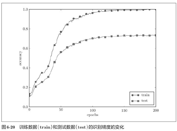

6.4.2 weight attenuation

Weight attenuation is a method often used to suppress over fitting. This method suppresses over fitting by punishing large weights in the process of learning. Many over fitting occurs because the value of weight parameters is too large.

Now let's do the experiment. For the experiment just carried out, the applicationThe weight attenuation of is shown in the following figure:

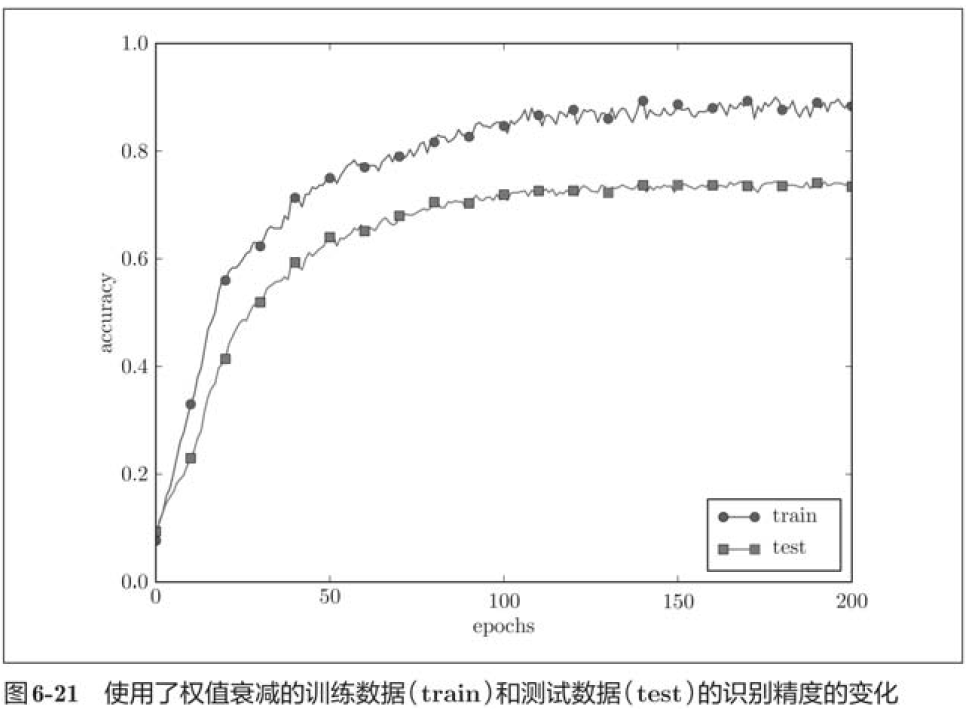
Although there is a gap between the recognition accuracy of training data and test data, compared with the results without weight attenuation, the gap becomes smaller, which shows that over fitting is restrained.

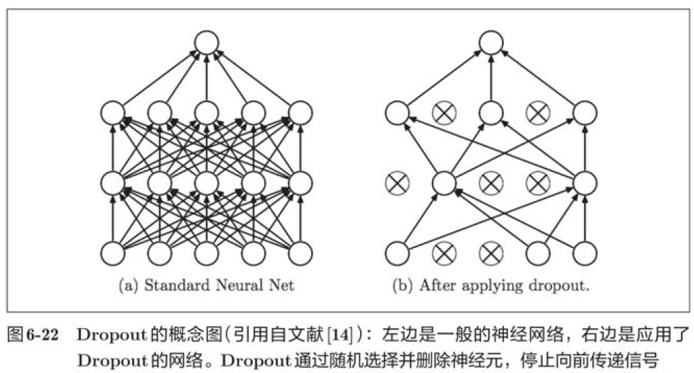
6.4.3 Dropout

Dropout is a method of randomly deleting neurons in the process of learning. During training, the neurons in the hidden layer are randomly selected and then deleted. The deleted neurons will no longer transmit signals. During training, every time the data is transmitted, the neurons to be deleted will be randomly selected. Then, during the test, although all neuron signals will be transmitted, the output of each neuron should be multiplied by the deletion ratio during training.

# coding: utf-8
import os
import sys
sys.path.append(os.pardir)  # Settings for importing files from the parent directory
import numpy as np
import matplotlib.pyplot as plt
from dataset.mnist import load_mnist
from common.multi_layer_net_extend import MultiLayerNetExtend
from common.trainer import Trainer

(x_train, t_train), (x_test, t_test) = load_mnist(normalize=True)

# In order to reproduce the over fitting, reduce the learning data
x_train = x_train[:300]
t_train = t_train[:300]

# Set whether to use Dropuout and the scale========================
use_dropout = True  # False without Dropout
dropout_ratio = 0.2
# ====================================================

network = MultiLayerNetExtend(input_size=784, hidden_size_list=[100, 100, 100, 100, 100, 100],
                              output_size=10, use_dropout=use_dropout, dropout_ration=dropout_ratio)
trainer = Trainer(network, x_train, t_train, x_test, t_test,
                  epochs=301, mini_batch_size=100,
                  optimizer='sgd', optimizer_param={'lr': 0.01}, verbose=True)
trainer.train()

train_acc_list, test_acc_list = trainer.train_acc_list, trainer.test_acc_list

# Draw graphics==========
markers = {'train': 'o', 'test': 's'}
x = np.arange(len(train_acc_list))
plt.plot(x, train_acc_list, marker='o', label='train', markevery=10)
plt.plot(x, test_acc_list, marker='s', label='test', markevery=10)
plt.xlabel("epochs")
plt.ylabel("accuracy")
plt.ylim(0, 1.0)
plt.legend(loc='lower right')
plt.show()

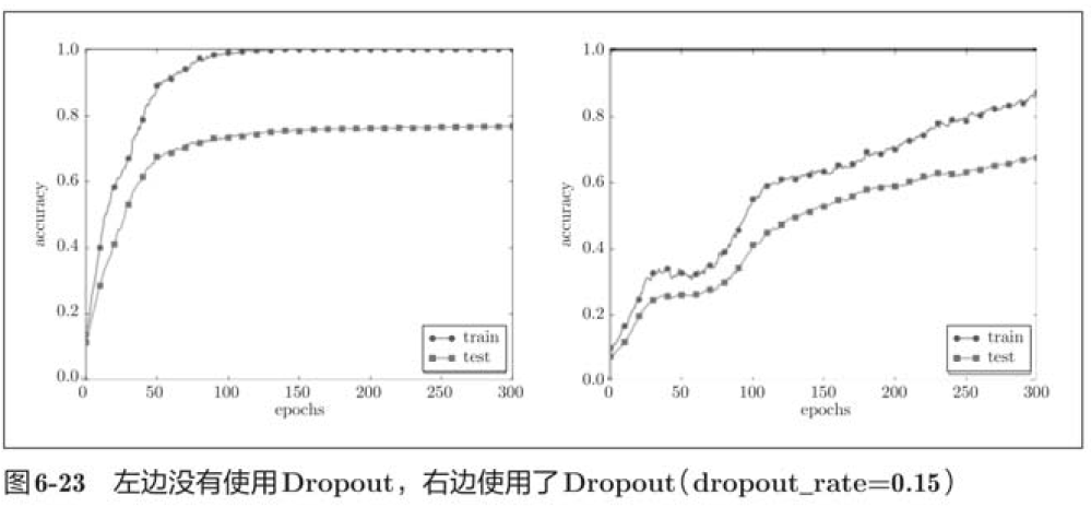In the above figure, by using Dropout, the difference between the recognition accuracy of training data and test data becomes smaller, and the recognition accuracy of training data does not reach 100%. Like this, by using Dropout, over fitting can be suppressed even in highly expressive networks.

Ensemble learning is often used in machine learning. The so-called integrated learning is to let multiple models learn separately, and then take the average value of the output of multiple models during reasoning. Through ensemble learning, the recognition accuracy of neural network can be improved by several percentage points. This integrated learning is closely related to Dropout, because Dropout can be understood as letting different models learn each time by randomly deleting neurons in the learning process. Moreover, when reasoning, the average value of the model can be obtained by multiplying the output of neurons by the deletion ratio. In other words, it can be understood that Dropout realizes the effect of integrated learning (simulated) through a network.

6.5 verification of super parameters

In neural networks, in addition to parameters such as weight and bias, hyperparameters often appear. The hyperparameters mentioned here refer to, for example, the number of neurons in each layer, the size of batch, the learning rate or weight attenuation during parameter update, etc. If these super parameters are not set with appropriate values, the performance of the model will be very poor. Although the value of super parameters is very important, there are usually many trials and errors in the process of determining super parameters.

6.5.1 validation data

Why not use test data to evaluate the performance of hyperparameters? This is because if the test data is used to adjust the superparameter, the value of the superparameter will fit the test data. In other words, using the test data to confirm the "good" or "bad" of the value of the superparameter will cause the value of the superparameter to be adjusted to fit only the test data. In this way, models that cannot fit other data and have low generalization ability may be obtained.

Therefore, when adjusting the super parameter, the special confirmation data for the super parameter must be used. The data used to adjust the super parameters is generally called validation data. We use this validation data to evaluate the quality of the hyperparameters.

The test data is used for the learning of parameters (weight and bias), and the verification data is used for the performance evaluation of super parameters. In order to confirm the generalization ability, the test data should be used at the end (ideally only once).

According to different data sets, some will be divided into three parts: training set, verification data and test data in advance, some will only be divided into two parts: training data and test data, and some will not be divided. In this case, users need to segment by themselves. If it is MNIST data set, the simplest way to obtain verification data is to divide 20% of the training data in advance as verification data.

6.5.2 optimization of super parameters

It is very important to gradually reduce the existence range of "good value" of hyperparameters when optimizing hyperparameters. The so-called gradual reduction of the range refers to roughly setting a range at the beginning, randomly selecting a super parameter (sampling) from this range, and using the sampled value to evaluate the recognition accuracy; Then, repeat the operation for many times, observe the result of recognition accuracy, and narrow the range of "good value" of super parameters according to the result. By repeating this operation, you can gradually confirm the appropriate range of super parameters.

Some reports show that the search method of random sampling is better than the regular search such as grid search when optimizing the super parameters of neural network. This is because among multiple super parameters, each super parameter has different influence on the final high recognition accuracy.

In the optimization of hyperparameters, it should be noted that deep learning takes a long time. Therefore, in the search of super parameters, we need to abandon those illogical super parameters as soon as possible. Therefore, in the optimization of hyperparameters, it is a good method to reduce the learning epoch and shorten the time required for one evaluation.

Briefly summarized as follows:

Step 0

Set the range of super parameters

Step 1

Random sampling from the set super parameter range

Step 2

Use the value of the super parameter sampled in step 1 for learning, and evaluate the recognition accuracy by verifying the data (but set the epoch to be very small)

Step 3

Repeat step 1 and step 2 (100 times, etc.) to narrow the range of super parameters according to the results of their recognition accuracy.

Repeat the above operations to continuously narrow the range of super parameters. When it is reduced to a certain extent, select a value of super parameters from the range, which is a method of optimizing super parameters.

6.5.3 realization of super parameter optimization

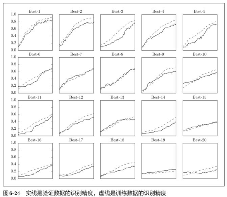The above figure shows the learning changes of verification data in the order of recognition accuracy from high to low. The learning rate is 0.001 to 0.01, and the weight attenuation coefficient isreachBetween, learning can proceed smoothly. In this way, observing the range of super parameters that can make learning go smoothly, so as to reduce the range of values, and then repeat the same operation in this reduced range, so as to reduce to the existence range of appropriate super parameters, and then select a final value of super parameters at a certain stage.

import sys, os
sys.path.append(os.pardir)
import numpy as np
import matplotlib.pyplot as plt
from dataset.mnist import load_mnist
from common.multi_layer_net import MultiLayerNet
from common.util import shuffle_dataset
from common.trainer import Trainer

(x_train, t_train), (x_test, t_test) = load_mnist(normalize=True)

# In order to achieve high speed and reduce training data
x_train = x_train[:500]
t_train = t_trian[:500]

# Split validation data
validation_rate = 0.20
validation_num = int(x_train.shape[0] * validation_rate)
x_train, t_train = shuffle_dataset(x_train, t_train)
x_val = x_train[:validation_num]
t_val = t_train[:validation_num]
x_train = x_train[validation_num:]
t_train = t_train[validation_num:]


def __train(lr, weight_decay, epocs=50):
    network = MultiLayerNet(input_size=784, hidden_size_list=[100, 100, 100, 100, 100, 100], output_size=10, weight_decay_lambda=weight_decay)
    trainer = Trainer(network, x_train, t_train, x_val, t_val, epochs=epocs, mini_batch_size=100, optimizer='sgd', optimizer_param={'lr':lr}, verbose=False)
    trainer.train()

    return trainer.test_acc_list, trainer.train_acc_list


# Random search of hyperparameters======================================
optimization_trial = 100
results_val = {}
results_train = {}
for _ in range(optimization_trial):
    # Specifies the range of the superparameters to search for=================
    weight_decay = 10 ** np.random.uniform(-8, -4)
    lr = 10 ** np.random.uniform(-6, -2)
    #================================================

    val_acc_list, train_acc_list = __train(lr, weight_decay)
    print('val acc:' + str(val_acc_list[-1]) + ' | lr:' + str(lr) + ', weight decay:' + str(weight_decay))
    key = 'lr:' + str(lr) + ', weight decay:' + str(weight_decay)
    results_val[key] = val_acc_list
    results_train[key] = train_acc_list

#Draw graphics==============================================
print('============ Hyper-Parameter Optimization Result ============')
grap_draw_num = 20
col_num = 5
row_num = int(np.ceil(grap_draw_num / col_num))
i = 0

for key, val_acc_list in sorted(results_val.items(), key=lambda x:x[1][-1], reverse=True):
    print('Best-' + str(i+1) + '(val acc:' + str(val_acc_list[-1]) + ') |' + key)

    plt.subplot(row_num, col_num, i+1)
    plt.title('Best-' + str(i+1))
    plt.ylim(0.0, 1.0)
    if i % 5: plt.yticks([])
    plt.xticks([])
    x = np.arange(len(val_acc_list))
    plt.plot(x, val_acc_list)
    plt.plot(x, results_train[key], '---')
    i += 1

    if i >= graph_draw_num:
        break

plt.show()

6.6 summary

In this chapter, we introduce several important skills in the learning of neural networks, such as the updating method of parameters, the assignment method of initial value of weights, Batch Normalization, Dropout, etc., which are indispensable technologies in modern neural networks. In addition, the skills introduced here are also frequently used in the most advanced in-depth learning.

1. Parameter updating methods include Momentum, AdaGrad, Adam and other methods in addition to SGD;

2. The assignment method of the initial value of weight is very important for correct learning;

3. As the initial value of weight, Xavier initial value and He initial value are more effective;

4. By using Batch Normalization, you can accelerate learning and become robust to initial values;

5. Regularization techniques to suppress over fitting include weight attenuation, Dropout, etc;

6. Gradually narrowing the scope of "good value" is an effective method to search for super parameters.

Topics: Python AI Deep Learning

Programmer Think