7.2 k-fold cross validation model performance
This method can solve the problem of over adaptation,
library(modeldata)
library(e1071)
data(mlc_churn)
churnTrain <- mlc_churn
ind <- cut(1:nrow(churnTrain), breaks = 10, labels = F)
accuracies <- c()
for (i in 1:10) {
  fit <- svm(churn~.,churnTrain[ind!=i,])
  predictions <- predict(fit, churnTrain[ind==i,!names(churnTrain) %in% c("churn")])
  correct_count <- sum(as.data.frame(predictions) == churnTrain[ind==i,c("churn")])
  accuracies <- append(correct_count/nrow(churnTrain[ind==i,]),accuracies)
}
accuracies
[1] 0.920 0.874 0.906 0.902 0.874 0.890 0.884 0.904 0.922 0.902
7.3 cross validation of e1071 package
# e1071 cross validation
library(e1071)
churnTrain <- churn[,!names(churn) %in% c('state',
                                          'area_code', "account_length")]
set.seed(2)
ind <- sample(2,nrow(churnTrain),replace = TRUE,
              prob = c(0.7,0.3))
trainset <- churnTrain[ind==1,]
testset <- churnTrain[ind==2,]
tuned <- tune.svm(churn~., data = trainset, gamma = 10^-2,
                  cost = 10^2, tunedcontrol = tune.control(cross = 10))
summary(tuned)
# Error estimation of 'svm' using 10-fold cross validation: 0.07473914
tuned$performances
  gamma cost      error dispersion
1  0.01  100 0.07473914 0.01605983
svmfit <- tuned$best.model
table(trainset[,c("churn")], predict(svmfit))
       yes   no
  yes  400   93
  no    14 2972
The tune function uses the wind format search method to complete parameter optimization. View other optimization functions? tune
7.4 cross validation of caret package
# caret
library(caret)
# Repeat 3 times with 10 fold cross
control <- trainControl(method = "repeatedcv",number = 10,
                        repeats = 3)
model <- train(churn~.,data = trainset, method = "rpart",
               preProcess="scale", trControl=control)
model
CART

3479 samples
  19 predictor
   2 classes: 'yes', 'no'

Pre-processing: scaled (69)
Resampling: Cross-Validated (10 fold, repeated 3 times)
Summary of sample sizes: 3131, 3132, 3130, 3130, 3131, 3132, ...
Resampling results across tuning parameters:

  cp          Accuracy   Kappa
  0.04056795  0.9301563  0.6720876
  0.05578093  0.9147378  0.5774005
  0.07505071  0.8731365  0.2416613

Accuracy was used to select the optimal model using the largest value.
The final value used for the model was cp = 0.04056795.
trainControl can set resampling parameters, and specify boot\boot632\cv\repeatdcv\LOOCV\LGOCV\non\oob\adaptive_cv\adaptive_boot\adaptive_LGOCV et al.
7.5 importance ranking of variables by caret package
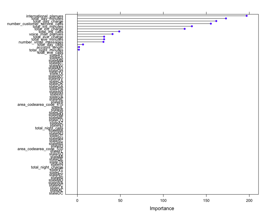
After the supervised learning model is obtained, the input value can be changed and the sensitivity of the output effect of a given model can be compared to evaluate the importance of different features to the model.
# Importance ranking
importance <- varImp(model, scale = FALSE)
importance
rpart variable importance

  only 20 most important variables shown (out of 69)

                              Overall
international_planyes         196.919
total_day_minutes             172.870
total_day_charge              161.582
number_customer_service_calls 155.274
total_intl_minutes            133.221
total_intl_charge             124.817
total_intl_calls               48.700
voice_mail_planyes             40.912
total_eve_charge               31.116
total_eve_minutes              31.116
...
plot(importance)
The objects generated from the training model in some classification algorithm packages such as extended rpart contain the importance of variables, which can be viewed and output.
library(rpart)
model.rp <- rpart(churn~.,data = trainset)
model.rp$variable.importance
             total_day_charge             total_day_minutes                         state
                   161.951011                    161.951011                     85.145010
           total_intl_minutes number_customer_service_calls             total_intl_charge
                    80.504234                     76.323349                     75.141041
...
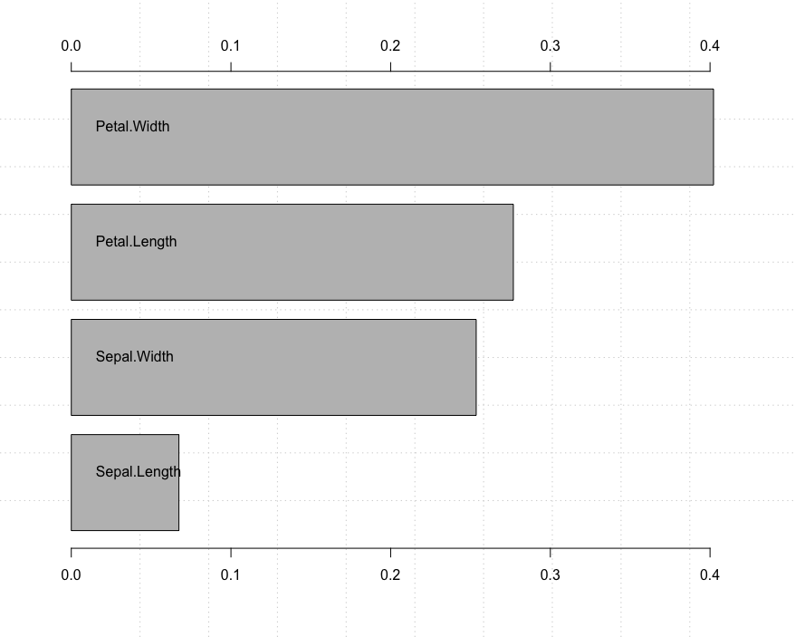
7.6 rimier package to sort the importance of variables
This takes a lot of effort. It seems that only numerical variables can do it.
# rminier
install.packages("rminer")
library(rminer)
model <- fit(Species~., iris,model = "svm")
variable.importance <- Importance(model,iris,method = "sensv")
L=list(runs=1,sen=t(variable.importance$imp),sresponses=variable.importance$sresponses)
mgraph(L,graph = "IMP",leg = names(iris),col = "gray", Grid = 4)
7.7 caret packages find highly correlated features
Remove the non numerical attributes, calculate the correlation to obtain a correlation matrix, set the threshold to 0.75, and select the highly correlated attributes.
# findCorrelation
new_train <- trainset[,!names(trainset) %in% c('churn',
                                     'international_plan', "voice_mail_plan")]
cor_mat <- cor(new_train)
highlyCorrelated <- findCorrelation(cor_mat, cutoff = 0.75)
names(new_train)[highlyCorrelated]
[1] "total_night_minutes" "total_intl_charge"   "total_day_charge"    "total_eve_charge"
You can also use the leaps, genetic and annual functions in the subselect package to achieve the same effect.
7.8 feature selection using caret package
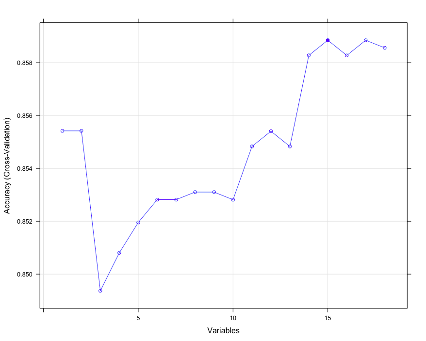
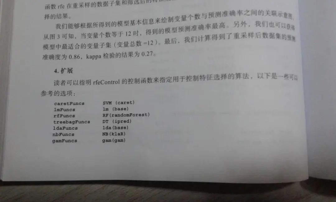
Feature selection can select the attribute subset with the lowest prediction error, which helps us to judge which features should be used to establish an accurate model. Recursive feature exclusion function rfe can automatically select the required features.
# caret selection feature
library(modeldata)
library(caret)
data(mlc_churn)
churnTrain <- mlc_churn
ind <- sample(2,nrow(churnTrain),replace = TRUE,
              prob = c(0.7,0.3))
trainset <- churnTrain[ind==1,]
testset <- churnTrain[ind==2,]
# Feature transformation should be that yes no changes to 1, 0, and factor changes to binary attribute
intl_plan <- model.matrix(~ trainset.international_plan - 1,
                          data = data.frame(trainset$international_plan))
colnames(intl_plan) <- c("trainset.international_planno"="intl_no",
                         "trainset.international_planyes"="intl_yes")

voice_plan <- model.matrix(~ trainset.voice_mail_plan - 1,
                           data = data.frame(trainset$voice_mail_plan))
colnames(voice_plan) <- c("trainset.voice_mail_planno"="voice_no",
                          "trainset.voice_mail_planyes"="voice_yes")
trainset$international_plan <- NULL
trainset$voice_mail_plan <- NULL
trainset <- cbind(intl_plan, voice_plan,trainset)
# testset does the same
intl_plan <- model.matrix(~ testset.international_plan - 1,
                          data = data.frame(testset$international_plan))
colnames(intl_plan) <- c("testset.international_planno"="intl_no",
                         "testset.international_planyes"="intl_yes")

voice_plan <- model.matrix(~ testset.voice_mail_plan - 1,
                           data = data.frame(testset$voice_mail_plan))
colnames(voice_plan) <- c("testset.voice_mail_planno"="voice_no",
                          "testset.voice_mail_planyes"="voice_yes")
testset$international_plan <- NULL
testset$voice_mail_plan <- NULL
testset <- cbind(intl_plan, voice_plan,testset)
# Linear discriminant analysis creates a feature screening algorithm, cross validation method cv
ldaControl <- rfeControl(functions = ldaFuncs, method = "cv")
# Reverse feature filtering
ldaProfile <- rfe(trainset[,names(trainset)!='churn'][,-c(5,6,7)],
                  trainset[,'churn'],sizes = c(1:18), rfeControl = ldaControl)
ldaProfile

Recursive feature selection

Outer resampling method: Cross-Validated (10 fold)

Resampling performance over subset size:

 Variables Accuracy   Kappa AccuracySD KappaSD Selected
         1   0.8554 0.02245   0.009841 0.06008
         2   0.8554 0.02245   0.009841 0.06008
         3   0.8494 0.23064   0.013363 0.10679
...
plot(ldaProfile, type = c("o","g"))
# Optimal variable subset
ldaProfile$optVariables
# Appropriate model
ldaProfile$fit
Call:
lda(x, y)

Prior probabilities of groups:
      yes        no
0.1417074 0.8582926

Group means:
postResample(predict(ldaProfile, testset[,names(testset)!="churn"]), testset[,c("churn")])
 Accuracy     Kappa
0.8520710 0.2523709
extend
7.9 evaluating the performance of regression model
Root mean square error method RMSE, relative square difference RSE, determination coefficient R-Square.
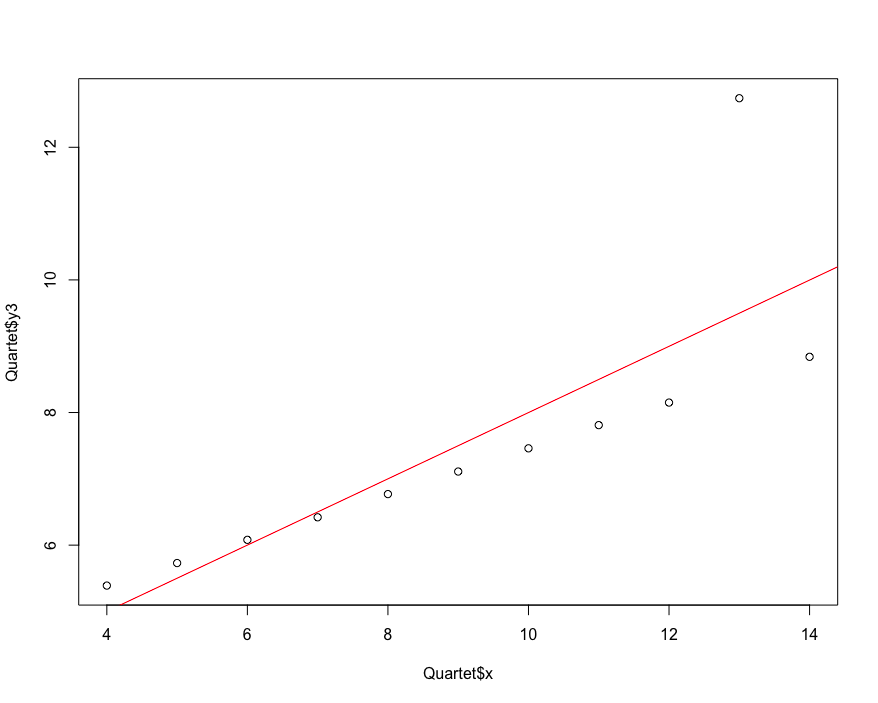
# Performance evaluation of regression model
library(car)
data("Quartet")
plot(Quartet$x,Quartet$y3)
lmfit<- lm(Quartet$y3~Quartet$x)
abline(lmfit, col="red")
predicted <- predict(lmfit,newdata = Quartet[c("x")])
actual <- Quartet$y3
# The function of caret package used here. This package is a treasure. It has everything
rmse <- RMSE(predicted, actual)
mu <- mean(actual)
rse <- mean((predicted-actual)^2)/mean((mu-actual)^2)
Rsquare <- 1-rse
c(rmse,rse,Rsquare)
[1] 1.118286 0.333676 0.666324
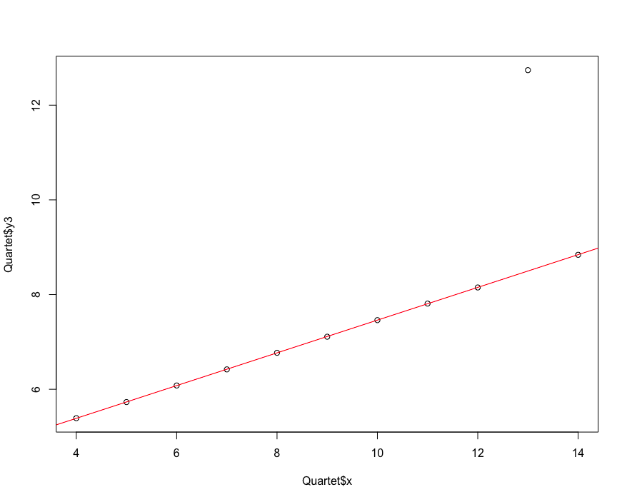
# MASS package rlm recalculation
library(MASS)
plot(Quartet$x,Quartet$y3)
rlmfit <- rlm(Quartet$y3~Quartet$x)
abline(rlmfit,col='red')
predicted <- predict(rlmfit, newdata = Quartet['x'])
rmse <- (mean((predicted-actual)^2))^0.5
rse <- mean((predicted-actual)^2)/mean((mu-actual)^2)
rsqure <- 1-rse
c(rmse,rse,Rsquare)
[1] 1.2790448 0.4365067 0.6663240
extend
library(e1071)
tune(lm,y3~x,data = Quartet)
Error estimation of 'lm' using 10-fold cross validation: 2.351897
Cross validation function of dacv.train LM can achieve the same effect
7.10 using confusion matrix to evaluate the prediction ability of the model
The accuracy, recall, specificity and accuracy of the model
# Confusion matrix
svm.model <- train(churn~., data=trainset,method = "svmRadial")
svm.pred <- predict(svm.model, testset[,names(testset)!="churn"])
table(svm.pred, testset[,"churn",drop=TRUE])
svm.pred  yes   no
     yes   12    1
     no   198 1290
confusionMatrix(svm.pred,testset[,"churn",drop=TRUE])
Confusion Matrix and Statistics

          Reference
Prediction  yes   no
       yes   12    1
       no   198 1290

               Accuracy : 0.8674
                 95% CI : (0.8492, 0.8842)
    No Information Rate : 0.8601
    P-Value [Acc > NIR] : 0.2183

                  Kappa : 0.0928
7.11 prediction ability of ROCR evaluation model
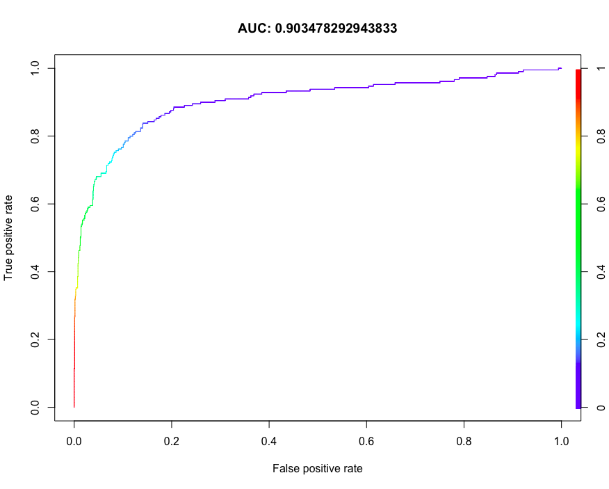
The receiver operating curve ROC is a common performance display graph of binary classification system. The true Yang and false Yang rates of different tangent points are marked on the curve. The classification performance of the model is usually measured based on the area under the curve AUC.
install.packages("ROCR")
library(ROCR)
svmfit <- svm(churn~.,data = trainset, prob = TRUE)
pred <- predict(svmfit, testset[,names(testset)!="churn"],probability = TRUE)
# Probability of marking yes
pred.prob <- attr(pred,"probabilities")
pred.to.roc <- pred.prob[, 2]
# forecast
pred.rocr <- prediction(pred.to.roc, testset$churn)
# Performance evaluation
perf.rocr <- performance(pred.rocr, measure = "auc", x.measure = "cutoff")
perf.tpr.rocr <- performance(pred.rocr, "tpr", "fpr")
plot(perf.tpr.rocr, colorize = T, main = paste("AUC:", (perf.rocr@y.values)))
7.12 compare ROC curves using caret package
install.packages("pROC")
library(pROC)
# Repeat 3 times with 10 fold cross
control <- trainControl(method = "repeatedcv", number = 10,
                        repeats = 3,classProbs = TRUE,
                        summaryFunction = twoClassSummary)
# glm classification
glm.model <- train(churn ~., data = trainset,method = "glm",
                   metric = "ROC", trControl = control)
# svm classification
svm.model <- train(churn ~., data = trainset,method = "svmRadial",
                   metric = "ROC", trControl = control)
rpart.model <- train(churn ~., data = trainset,method = "rpart",
                     metric = "ROC", trControl = control)
# Forecast separately
glm.probs <- predict(glm.model, testset[,names(testset) != "churn"], type = "prob")
svm.probs <- predict(svm.model, testset[,names(testset) != "churn"], type = "prob")
rpart.probs <- predict(rpart.model, testset[,names(testset) != "churn"], type = "prob")
# Generate ROC curve in a graph
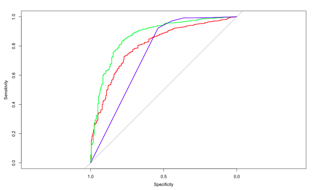
glm.ROC <- roc(response = testset[,c("churn"),drop=TRUE],
               predictor = glm.probs$yes,
               levels = levels(testset[,"churn",drop=TRUE]))
plot(glm.ROC, type = "S", col = 'red')

svm.ROC <- roc(response = testset[,c("churn"),drop=TRUE],
               predictor = svm.probs$yes,
               levels = levels(testset[,"churn",drop=TRUE]))
plot(svm.ROC, add = TRUE, col = 'green')
rpart.ROC <- roc(response = testset[,c("churn"),drop=TRUE],
               predictor = rpart.probs$yes,
               levels = levels(testset[,"churn",drop=TRUE]))
plot(rpart.ROC, add = TRUE, col = 'blue')
Error in colnames (data): argument "data" is missing, with no default. Finally, if it is found that tibble does not reduce the dimension by default, add drop=TRUE to solve it.
7.13 performance differences of caret package comparison model
# Model resampling
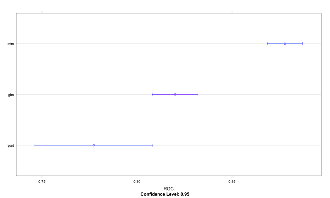
cv.values <- resamples(list(glm=glm.model, svm=svm.model, rpart = rpart.model))
summary(cv.values)
Call:
summary.resamples(object = cv.values)

Models: glm, svm, rpart
Number of resamples: 30

ROC
           Min.   1st Qu.    Median      Mean   3rd Qu.      Max. NA's
glm   0.7483007 0.7977494 0.8187351 0.8200275 0.8357939 0.8953608    0
svm   0.8356721 0.8594691 0.8722842 0.8778421 0.9018812 0.9184929    0
rpart 0.6446078 0.7146965 0.7666979 0.7773052 0.8459407 0.9173395    0

Sens
           Min.   1st Qu.    Median      Mean   3rd Qu. Max. NA's
glm   0.1600000 0.2088235 0.2672549 0.2667320 0.3184314 0.40    0
svm   0.2600000 0.3879412 0.4454902 0.4460654 0.5049020 0.66    0
rpart 0.2352941 0.3800000 0.4411765 0.4622876 0.5637255 0.76    0

Spec
           Min.   1st Qu.    Median      Mean   3rd Qu.      Max. NA's
glm   0.9509804 0.9639639 0.9673203 0.9666242 0.9705882 0.9771242    0
svm   0.9346405 0.9542484 0.9672131 0.9641094 0.9729749 0.9836601    0
rpart 0.9705882 0.9836601 0.9901639 0.9885492 0.9934641 1.0000000    0
dotplot(cv.values, metric = "ROC")
bwplot(cv.values, layout=c(3,1))
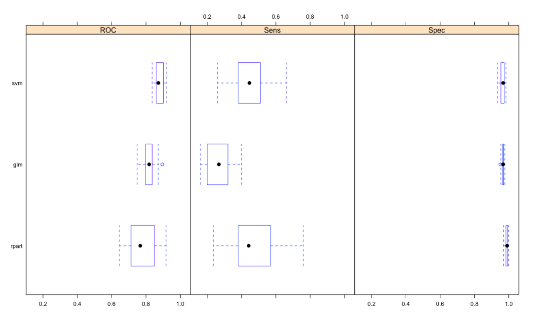
Extensions can also use densityplot Splom and xyplot function visualization