The prediction results of multiple classifiers are combined to obtain the final decision, so as to obtain better classification and regression performance. A single classifier is only suitable for a specific type of data, so it is difficult to ensure the best classification model. If the prediction results of different algorithms are averaged, a better classification model may be obtained compared with one classifier. bagging, boosting and random forest are the three most widely used ensemble learning algorithms.
- bagging: voting algorithm. Firstly, bootstrap generates different training data sets, then obtains multiple basic classifiers, and finally combines them to obtain a relatively better model.
- Boosting: similar to bagging, the difference is that boosting is carried out in sequence. The latter round of classifier is related to the results of the previous classifier, that is, learning on the basis of misclassification and compensating learning.
- Random forest: a classifier containing multiple decision trees. The classification results are obtained by voting. A separate classification decision tree is generated for each type of feature vector. From these classification results, multiple decision trees with the highest number of votes are selected to complete the classification, or an average value is selected as the output of regression processing.
8.2 data classification using bagging method
adabag package supports both bagging and boosting methods. The former is Breman bagging algorithm (version classifier theory is proposed for the first time).
install.packages("adabag")
library(adabag)
# find

data(iris)
churnTrain <- iris
ind <- sample(2,nrow(churnTrain),replace = TRUE,
              prob = c(0.7,0.3))
trainset <- churnTrain[ind==1,]
testset <- churnTrain[ind==2,]
set.seed(2)
churn.bagging <- bagging(churn~., data = trainset, mfinal = 10) #The number of iterations is 10
churn.bagging$importance
Petal.Length  Petal.Width Sepal.Length  Sepal.Width
    75.53879     24.46121      0.00000      0.00000
 churn.predbagging$confusion
               Observed Class
Predicted Class setosa versicolor virginica
     setosa         18          0         0
     versicolor      0         19         0
     virginica       0          2        15
churn.baggingcv$error
[1] 0.03703704
The algorithm is derived from Bootstrap aggregation. It has the advantages of stability, accuracy, powerful function and easy implementation. It is often used in data classification and regression processing. The algorithm is defined as follows: given a data set of size n, m new data sets Di are obtained through bootstrap sampling, M models are obtained through M samples, and then the optimal model is obtained. The disadvantage is that the results are difficult to explain. The extended ipred package can also achieve the same function. After testing, it is very fast. It hasn't been moving for half an hour. There should be no cross validation.
churn.bagging <- bagging(churn~., data = trainset, coob=TRUE)
churn.bagging
Bagging classification trees with 25 bootstrap replications

Call: bagging.data.frame(formula = churn ~ ., data = trainset, coob = TRUE)

Out-of-bag estimate of misclassification error:  0.0606
# Misclassification rate
mean(predict(churn.bagging)!=trainset$churn)
[1] 0.06115418
# forecast
churn.predction <- predict(churn.bagging, newdata = testset, type = "class")
prediction.table <- table(churn.predction, testset$churn)
prediction.table
churn.predction  yes   no
            yes  170   16
            no    57 1274
8.3 cross validation using bagging method
Evaluate the robustness of the classification model
# cv
churn.baggingcv <- bagging.cv(churn~., v = 10, data = trainset,
                              mfinal = 10)
# Error in bagging.cv(churn ~ ., v = 10, data = trainset, mfinal = 10) :
   v should be in [2, n] The problem of the original data set is used here iris replace
churn.baggingcv$confusion
               Observed Class
Predicted Class setosa versicolor virginica
     setosa         18          0         0
     versicolor      0         19         0
     virginica       0          2        15
# Misclassification rate
churn.predbagging$error
[1] 0.03703704
The churn dataset reports an error. Here, the iris simple dataset curve is used to report the country. The advantage is that it can save time.
8.4 data classification using boosting method
adabag implements AdaBoost and SANME algorithms.
# boosting
set.seed(2)
churn.boost <- boosting(Species~., data = trainset, mfinal = 3,
                        coeflearn = "Freund", boos = FALSE,
                        control=rpart.control(maxdepth=3))
churn.boost.pred <- predict.boosting(churn.boost, newdata = testset)
churn.boost.pred$confusion
churn.boost.pred$confusion
               Observed Class
Predicted Class setosa versicolor virginica
     setosa         18          0         0
     versicolor      0         20         1
     virginica       0          1        14
churn.boost.pred$error
[1] 0.03703704
The idea of boosting algorithm is to gradually optimize (change the weight) the weak classifier (such as a single decision tree) to become a strong classifier. Bagging and boosting both adopt the idea of integrated learning. The difference is that bagging combines independent models and boosting iterative learning. mfinal is the number of iterations, coeflearn is the control method of weight update coefficient, observation weight boos and rpart (single decision tree). extend
install.packages(c("mboost","ada"))
library(mboost)
library(pROC)
library(caret)
install.packages("MLmetrics")
set.seed(2)
ctrl <- trainControl(method = "repeatedcv", repeats = 1,
                     classProbs = TRUE,
                     summaryFunction = twoClassSummary)
ada.train <- train(churn~.,data = trainset, method = "ada",
                   metric = "ROC", trControl = ctrl)
#  Here iris reports an error and switches back to the churn dataset
  nu maxdepth iter       ROC      Sens        Spec      ROCSD     SensSD      SpecSD
1 0.1        1   50 0.8600045 0.9090204 0.010719176 0.03719839 0.05786791 0.007708342
...
plot(ada.train)
ada.predict <- predict(ada.train, testset, "prob")
ada.predict.result <- ifelse(ada.predict[1]>0.5, "yes", "no")
table(testset$churn, ada.predict.result)
     ada.predict.result
        no  yes
  yes   71  143
  no  1301    6
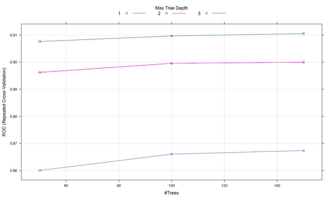
A rare figure in this chapter
8.5 cross validation using boosting method
churn.boostingcv <- boosting.cv(Species~., v=10, data = trainset,
            mfinal = 5, control = rpart.control(cp=0.01))
churn.boostingcv$confusion
               Observed Class
Predicted Class setosa versicolor virginica
     setosa         32          0         0
     versicolor      0         26         3
     virginica       0          3        32
churn.boostingcv$error
[1] 0.0625
8.6 use the gradient boosting method to classify the data
It is also to combine the weak classifiers together, and then get a new basic classifier when it is most correlated with the negative gradient of the loss function. It can be used for regression analysis and classification, and has good adaptability to different data sets.
# gradient boosting
install.packages("gbm")
library(gbm)
# The response value is 0 ~ 1, so it is converted
trainset$churn <- ifelse(trainset$churn =="yes", 1,0)
set.seed(2)
churn.gbm <- gbm(formula = churn ~ ., distribution = "bernoulli", data = trainset,
n.trees = 1000, interaction.depth = 7, shrinkage = 0.01,
cv.folds = 3) # Shrink step reduces the parameter, that is, learning speed; interaction.depth maximum depth of decision tree
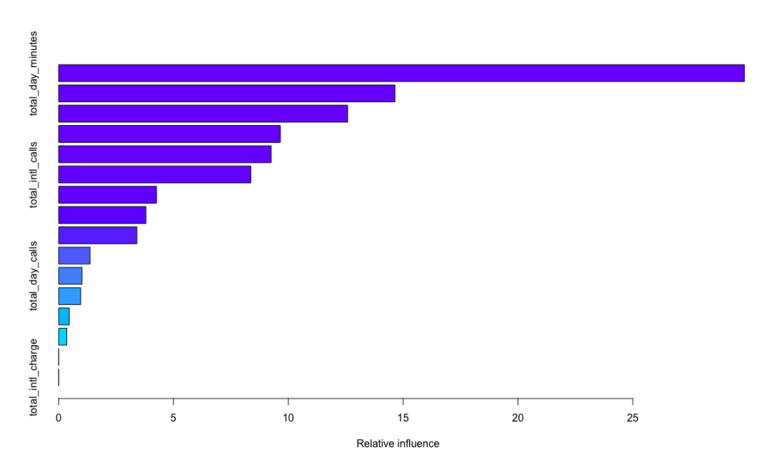
summary(churn.gbm)
var rel.inf
total_day_minutes total_day_minutes 29.8623601
total_eve_minutes total_eve_minutes 14.6407627
number_customer_service_calls number_customer_service_calls 12.5827527
total_intl_minutes total_intl_minutes 9.6529151
...
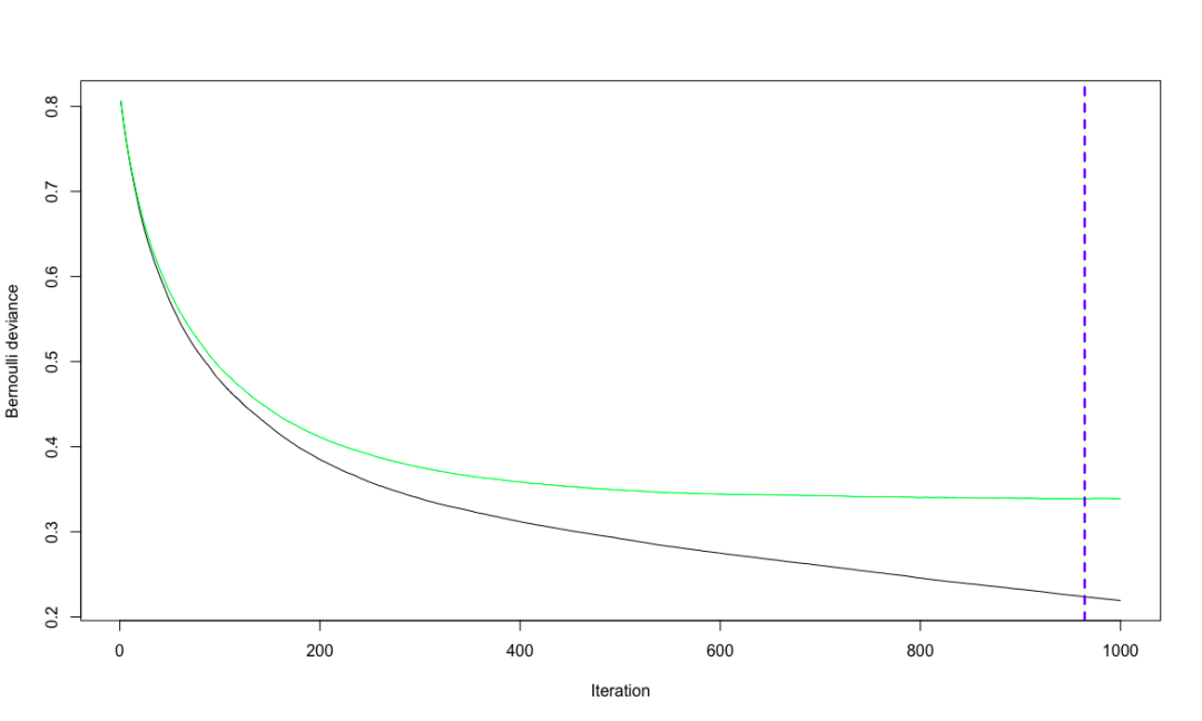
# Cross validation to determine the optimal number of iterations
churn.iter <- gbm.perf(churn.gbm, method = "cv")
# Logarithmic singularity of Bernoulli loss function
churn.predict <- predict(churn.gbm, testset, n.trees = churn.iter)
str(churn.predict)
num [1:1521] -3.56 -3.36 -2.99 -3.82 -3.52 ...
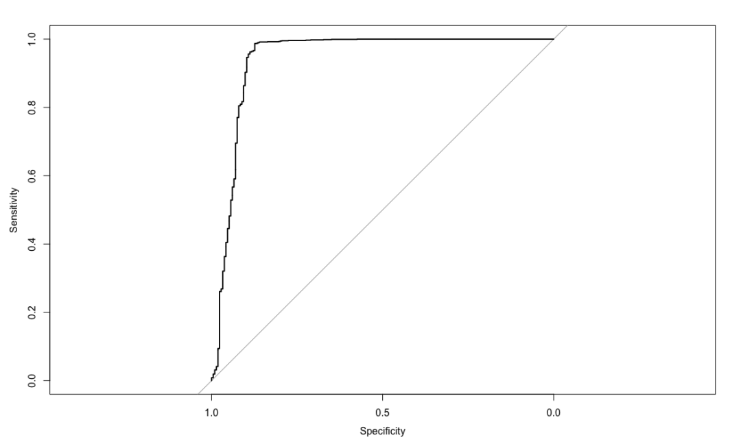
# ROC, get the best critical value of the maximum accuracy
# ROC
churn.roc <- roc(testset$churn, churn.predict)
plot(churn.roc)
# coords gets the best critical value
coords(churn.roc, "best")
threshold specificity sensitivity
1 -0.7369319 0.8738318 0.9869931
# coords gets the best critical value
coords(churn.roc, "best")
churn.predict.class <- ifelse(churn.predict >c(coords(churn.roc,"best")["threshold"]),
"yes","no")
table(testset$churn, churn.predict.class)
churn.predict.class
no yes
yes 27 187
no 1290 17
The idea of the algorithm is as follows: firstly, calculate the variance of the residual of each divided data set, and determine the optimal division of each stage accordingly. The selected model takes the variance processed in the previous stage as the learning goal to re model and reduce. Gradient descent is adopted, that is, change along the direction of derivative descent to minimize the residual variance. expand
library(mboost)
# It only supports numerical values, removal and conversion to non numerical values. It is found that the source of the previous error should be the conversion of yes and no. only adding a c() is OK. It is unscientific. no matter what, it can achieve the purpose
trainset$churn <- ifelse(trainset$churn ==c("yes"),1,0)
trainset$voice_mail_plan = NULL
trainset$international_plan = NULL
churn.mboost <- mboost(churn ~., data = trainset, control = boost_control(mstop = 10))
summary(churn.mboost)
  Model-based Boosting

Call:
mboost(formula = churn ~ ., data = trainset, control = boost_control(mstop = 10))


  Squared Error (Regression)

Loss function: (y - f)^2


Number of boosting iterations: mstop = 10
Step size:  0.1
Offset:  0.1417074
Number of baselearners:  14

Selection frequencies:
            bbs(total_day_minutes) bbs(number_customer_service_calls)
                               0.6                                0.4
par(mfrow=c(1,2))
plot(churn.mboost)
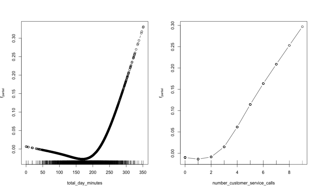
Local contribution of important attributes
Calculate classifier edge
boost.margins <- margins(churn.boost, trainset)
boost.pred.margins <- margins(churn.boost.pred, testset)
plot(sort(boost.margins[[1]]),
     (1:length(boost.margins[[1]]))/length(boost.margins[[1]]),
     type = 'l', xlim = c(-1,1),
     main = "Boosting:Magrin cumulative distribution graph",
     xlab = "margin", ylab = "% observations", col= 'blue')
lines(sort(boost.pred.margins[[1]]),
      (1:length(boost.pred.margins[[1]]))/length(boost.pred.margins[[1]]),
      type = "l", col="green")
abline(v=0, col='red', lty=2)
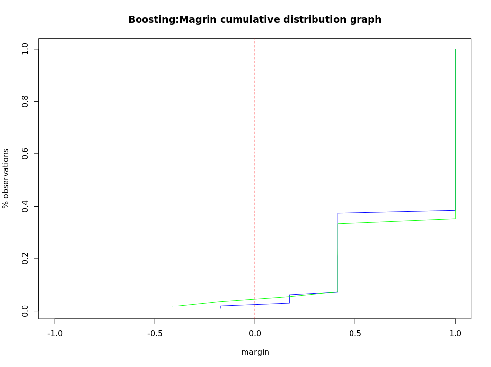
Edge cumulative distribution map of boosting classifier
# Percentage of negative edges that match training and test set errors
boosting.training.margin <- table(boost.margins[[1]]>0)
boosting.negative.training <- as.numeric(boosting.training.margin[1])/boosting.training.margin[2]
boosting.negative.training
     TRUE
0.0212766
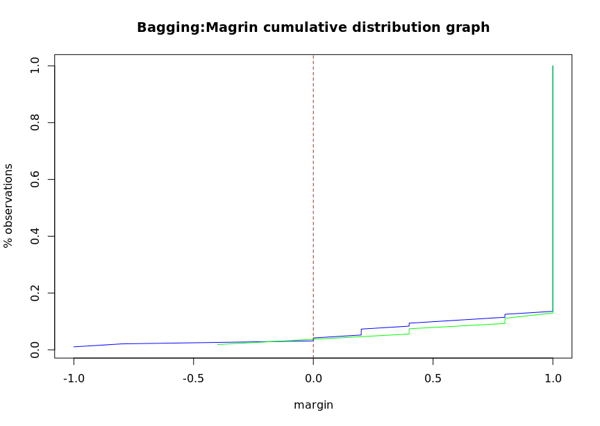
# Calculate the edge of bagging classifier
bagging.margins = margins(churn.bagging, trainset)
bagging.pred.margins <- margins(churn.predbagging,testset)
plot(sort(bagging.margins[[1]]),
     (1:length(bagging.margins[[1]]))/length(bagging.margins[[1]]),
     type = "l", xlim = c(-1,1),
     main = "Bagging:Magrin cumulative distribution graph",
     xlab = "margin", ylab = "% observations", col= 'blue')
lines(sort(bagging.pred.margins[[1]]),
      (1:length(bagging.pred.margins[[1]]))/length(bagging.pred.margins[[1]]),
      type = "l", col="green")
abline(v=0, col='red', lty=2)
# Similarly, calculate the percentage
bagging.training.margin <- table(bagging.margins[[1]]>0)
bagging.negative.training <- as.numeric(bagging.training.margin[1])/boosting.training.margin[2]
bagging.negative.training
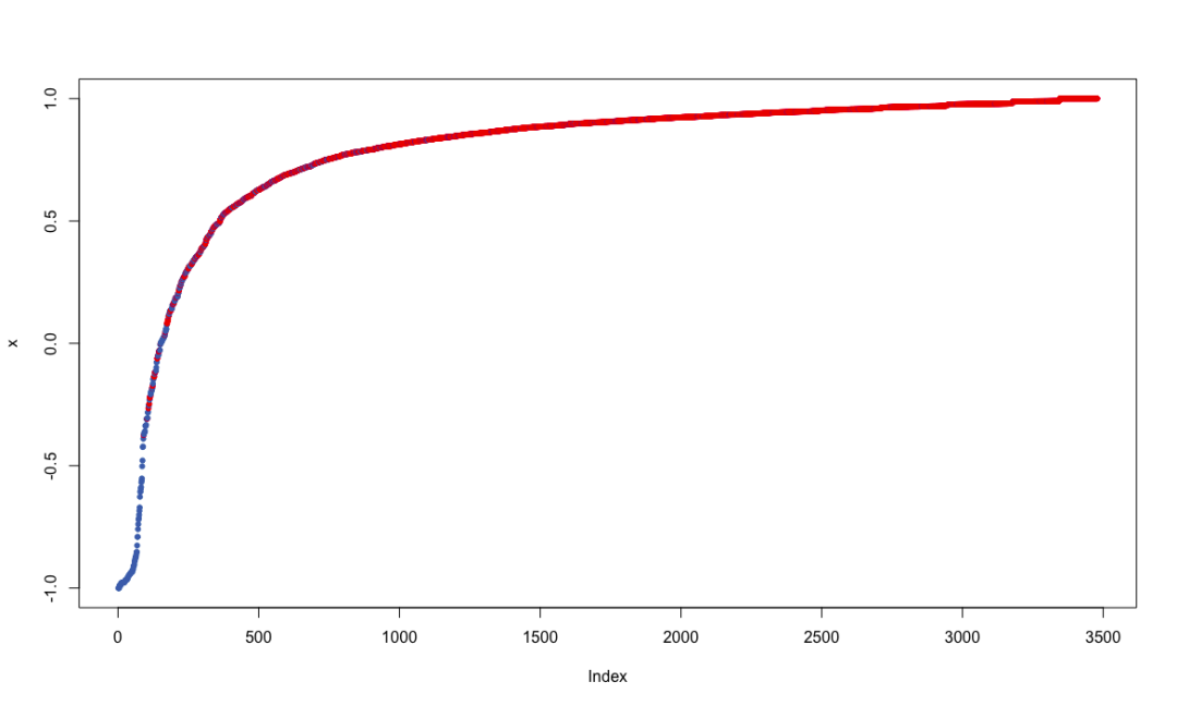
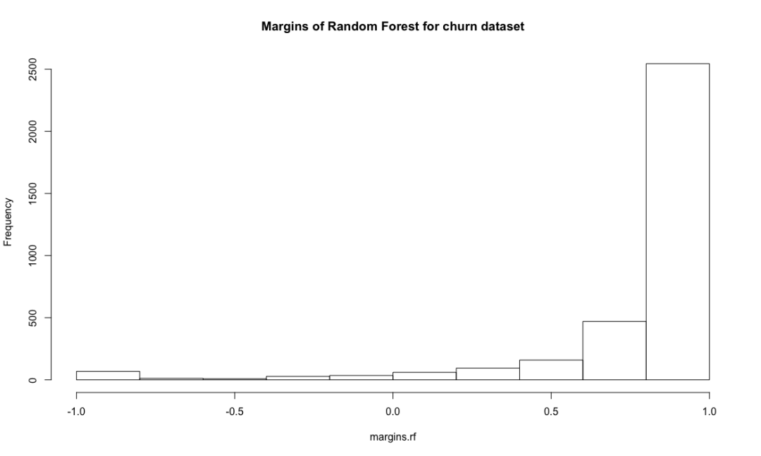
Edge is a measure of classifier certainty, which is calculated according to the number of classification samples and the maximum misclassification samples. Correctly classified samples establish edges, and incorrectly classified samples form negative edges. If the edges are close to 1, it indicates that the reliability of correctly classified samples is very high. Samples with uncertain classification have only small edges. The margin function can calculate AdaBoost The edges of M1, AdaBoost samme and bagging classifiers return an edge vector, which can draw an edge cumulative distribution curve to show the edge distribution. If each observation can be divided correctly, the distribution map will be a vertical line with an edge value of 1. Generally, the negative edge of the misclassification sample of the training data set is similar to that of the test data set.
Error evolution of computational ensemble classification algorithm
# Error evolution
boosting.evol.train <- errorevol(churn.boost, trainset)
boosting.evol.test <- errorevol(churn.boost, testset)
plot(boosting.evol.test$error, type = "l", ylim = c(0,1),
     main = "Boosting error versus number of trees",
     xlab = "Iteration", ylab = "Error", col='red',
     lwd=2)
lines(boosting.evol.train$error, cex = .5, col='blue',lty=2,
      lwd=2)
legend('topright', c('test','train'), col = c('red', 'blue'),
       lty = 1:2, lwd=2)
The errorevol function is provided in the adabag package to facilitate users to estimate the error of the integrated classification algorithm according to the number of iterations.

# bagging
# Error evolution
bagging.evol.train <- errorevol(churn.bagging, trainset)
bagging.evol.test <- errorevol(churn.bagging, testset)
plot(bagging.evol.test$error, type = "l", ylim = c(0,1),
     main = "Bagging error versus number of trees",
     xlab = "Iteration", ylab = "Error", col='red',
     lwd=2)
lines(bagging.evol.train$error, cex = .5, col='blue',lty=2,
      lwd=2)
legend('topright', c('test','train'), col = c('red', 'blue'),
       lty = 1:2, lwd=2)
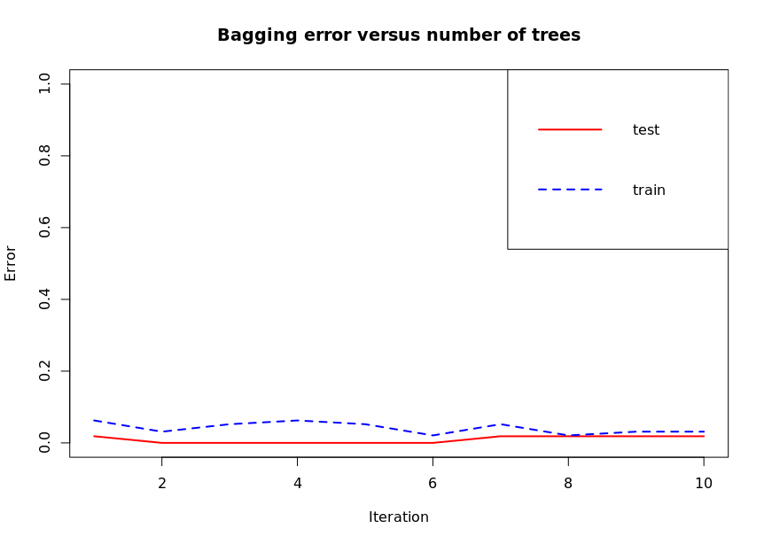
The figure shows the change of classification error after each iteration. Predict can be called Bagging and predict Boosting for pruning.
8.9 classification of random forest data
Multiple decision trees are generated in the training process, and each tree will generate prediction output according to the input. The voting mechanism is used to select the category mode as the prediction result.
# random Forest
install.packages("randomForest")
library(randomForest)
churn.rf <- randomForest(churn ~., data = trainset, importance=T) # Evaluate the importance of the predictor
churn.rf
Call:
randomForest(formula = churn ~ ., data = trainset, importance = T)
Type of random forest: classification
Number of trees: 500
No. of variables tried at each split: 4
OOB estimate of error rate: 4.31%
Confusion matrix:
yes no class.error
yes 363 130 0.263691684
no 20 2966 0.006697924
# Forecast classification
churn.prediction <- predict(churn.rf, testset)
table(churn.prediction, testset$churn)
churn.prediction yes no
yes 167 7
no 47 1300
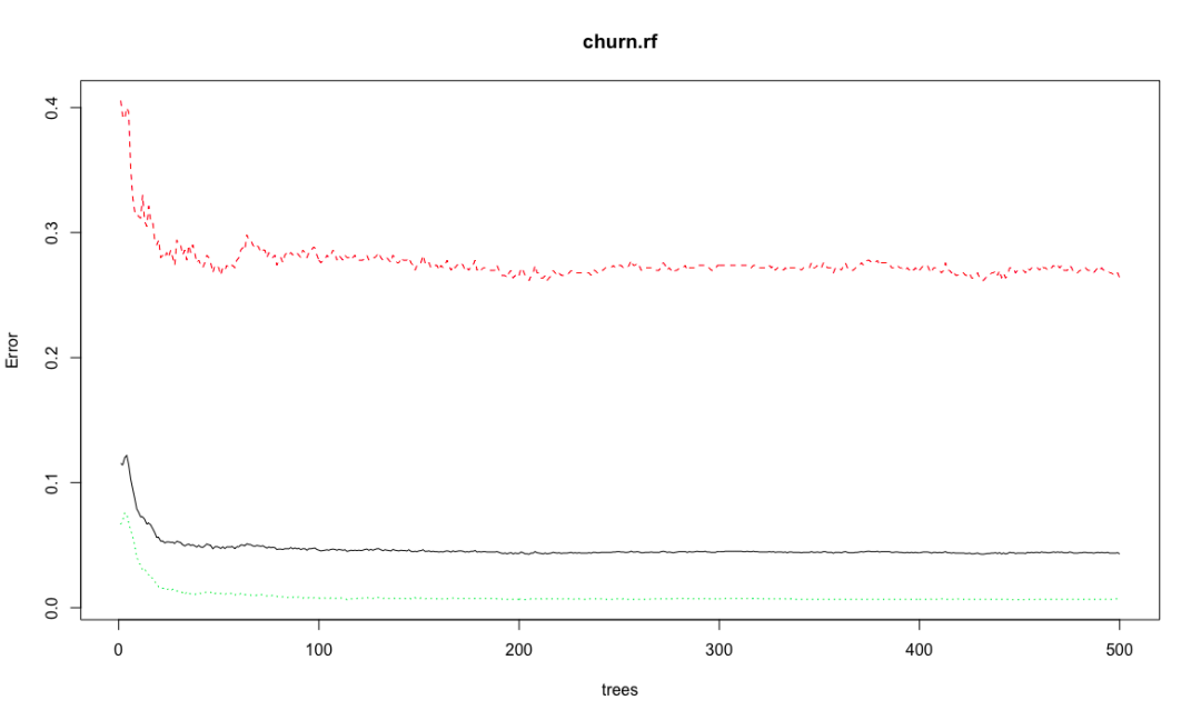
plot(churn.rf)
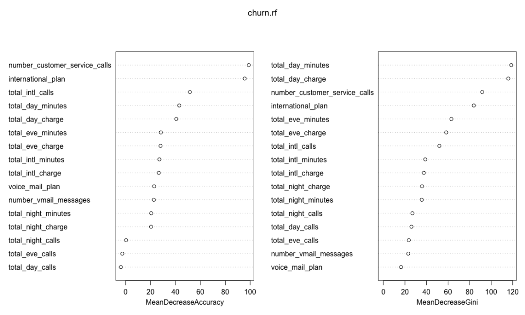
importance(churn.rf)
yes no MeanDecreaseAccuracy
international_plan 93.0223581 72.5504101 95.5848053
voice_mail_plan 22.5321109 18.2760474 22.8558091
number_vmail_messages 23.0980210 17.5029154 22.6011108
total_day_minutes 33.4914749 33.8653396 43.0515228
varImpPlot(churn.rf)
margins.rf <- margin(churn.rf, trainset)
plot(margins.rf)
hist(margins.rf, main = "Margins of Random Forest for churn dataset")
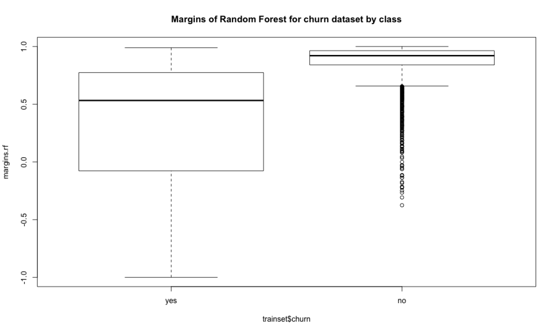
boxplot(margins.rf~ trainset$churn, main = "Margins of Random Forest for churn dataset by class")
Random forest combines multiple weak learning machines (decision trees) to get a strong learning machine. The processing process is very similar to bagging. First, boost sampling is used to find the prediction attribute that can provide the best segmentation effect. In case of regression, the average value or weighted average value of all predictions will be taken as the final output. In case of classification, select the category prediction mode as the final prediction. The algorithm includes two parameters: the number of ntree decision trees and the number of features that mtry can use to find the best features. Bagging algorithm only uses the former. If mtry = the eigenvalue of the training data set, the random forest is equivalent to bagging. The biggest advantage is that the calculation is easy and efficient, and the fault tolerance of missing data or unbalanced data is high; The main disadvantage is that the data beyond the training set can not be predicted, and it is easy to be affected by noise data, resulting in over adaptation. The cforest function of the extended cforest package can also implement the random forest algorithm
# expand
install.packages("party")
library(party)
churn.cforest <- cforest(churn~., data = trainset,
                         controls = cforest_unbiased(ntree=1000,mtry=5))
churn.forest.prediction <- predict(churn.cforest, testset, OOB=TRUE, type = "response")
table(churn.forest.prediction, trainset$churn) # This place is amazing. Let's put a question mark first

churn.forest.prediction  yes   no
                    yes  348   21
                    no   145 2965
8.10 estimating the prediction error of different classifiers
The cross validation of multiple classification algorithms using errorst function proves whether the integrated classifier is better than a single decision tree.
# ipred erroest
library(ipred)
churn.bagging <- errorest(churn ~., data = trainset, model = bagging);churn.bagging
Call:
errorest.data.frame(formula = churn ~ ., data = trainset, model = bagging)

  10-fold cross-validation estimator of misclassification error

Misclassification error:  0.052
library(ada)
churn.mboosting <- errorest(churn ~., data = trainset, model = ada);churn.mboosting
Call:
errorest.data.frame(formula = churn ~ ., data = trainset, model = ada)

  10-fold cross-validation estimator of misclassification error

Misclassification error:  0.048
hurn.rf <- errorest(churn~., data = trainset, model = randomForest);churn.rf
Call:
errorest.data.frame(formula = churn ~ ., data = trainset, model = randomForest)

  10-fold cross-validation estimator of misclassification error

Misclassification error:  0.0454
churn.tree <- errorest(churn~., data = trainset, model = rpart, predict=churn.predict);churn.tree
Call:
errorest.data.frame(formula = churn ~ ., data = trainset, model = rpart,
    predict = churn.predict)

  10-fold cross-validation estimator of misclassification error

Misclassification error:  0.0606
randomForest has the lowest misclassification rate, the best performance, the worst performance of a single tree, and integrated learning is better than a single tree. ada provides a method of boosting classification.