Objective: to complete the Titanic survival prediction based on the Titanic data set.

import pandas as pd
import numpy as np
import matplotlib.pyplot as plt
import seaborn as sns
from IPython.display import Image
plt.rcParams['font.sans-serif'] = ['SimHei']  
# Used to display Chinese labels normally
plt.rcParams['axes.unicode_minus'] = False  
# Used to display negative signs normally
plt.rcParams['figure.figsize'] = (10, 6)  
# Set output picture size
train = pd.read_csv('train.csv')#Original data
data = pd.read_csv('clear_data.csv')
data.head(10)#Load cleaned data

Screenshot of some data after cleaning:

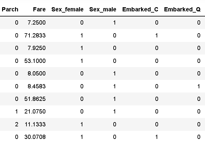
Compared with the original data, the cleared data lacks unimportant character variables such as name, ticket and cabin,
The information of gender and boarding port is transformed into 0-1 variables, which is more intuitive as a whole.

Model building

1. Cut training set and test set

from sklearn.model_selection import train_test_split
# Generally, x and y are taken out before cutting. In some cases, uncut ones will be used. At this time, x and y can be used. x is the cleaned data and Y is the survival data we want to predict, 'Survived'
X = data
y = train['Survived']
# Cut the dataset
X_train, X_test, y_train, y_test = train_test_split(X, y, stratify=y, random_state=0)
# View data shapes
X_train.shape, X_test.shape

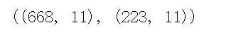
The function of stratify=y is to keep the data classification proportion of Y in the test set consistent with that in the whole data set. And random_state=0 ensures that random results can be repeated.

 2. Model creation

The model is divided into linear model based classification model (logistic regression) and tree based classification model (decision tree, random forest).

from sklearn.linear_model import LogisticRegression
from sklearn.ensemble import RandomForestClassifier
lr = LogisticRegression()
lr.fit(X_train, y_train)
#Default parameter logistic regression model
# View training set and test set score values
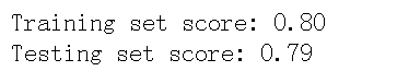
print("Training set score: {:.2f}".format(lr.score(X_train, y_train)))
print("Testing set score: {:.2f}".format(lr.score(X_test, y_test)))

train set is used to train the model and estimate parameters.

test set is used to test and evaluate the quality of the trained model, not for the training model.

# Logistic regression model after adjusting parameters
lr2 = LogisticRegression(C=100)
lr2.fit(X_train, y_train)
print("Training set score: {:.2f}".format(lr2.score(X_train, y_train)))
print("Testing set score: {:.2f}".format(lr2.score(X_test, y_test)))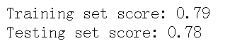

 

# Random forest classification model with default parameters
rfc = RandomForestClassifier()
rfc.fit(X_train, y_train)
print("Training set score: {:.2f}".format(rfc.score(X_train, y_train)))
print("Testing set score: {:.2f}".format(rfc.score(X_test, y_test)))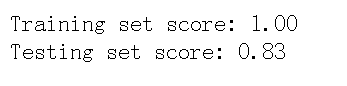

 

# Stochastic forest classification model with adjusted parameters
rfc2 = RandomForestClassifier(n_estimators=100, max_depth=5)
rfc2.fit(X_train, y_train)
print("Training set score: {:.2f}".format(rfc2.score(X_train, y_train)))
print("Testing set score: {:.2f}".format(rfc2.score(X_test, y_test)))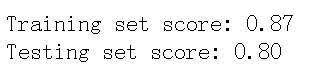

3. Output model prediction results

The general supervision model has a predict in sklearn, which can output the prediction tag_ Proba can output label probability.

# Forecast label
pred = lr.predict(X_train)
pred[:10]

# Predicted tag probability
pred_proba = lr.predict_proba(X_train)
pred_proba[:10]

 

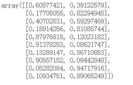
Survival can be divided into 0 and 1. So the prediction tag is 0 or 1. In the prediction tag probability, each row corresponds to a piece of prediction data, and the two columns correspond to the prediction probability for 0 and 1 respectively. The sum of probability is 1. Take the category with the highest probability as the prediction result of the sample. For example, in the first line, 0.60877 > 0.39122, so the prediction result is 0.

Model evaluation

• Model evaluation is to know the generalization ability of the model.
• Cross validation is a statistical method to evaluate generalization performance. It is more stable and comprehensive than the method of dividing training set and test set.
• In cross validation, the data is divided many times and multiple models need to be trained.
• The most commonly used cross validation is k-fold cross validation, where k is the number specified by the user, usually 5 or 10.
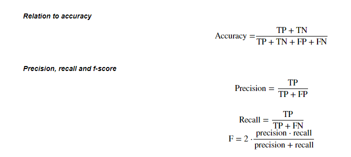
• Accuracy measures how many samples are predicted to be positive examples
• recall measures how many positive samples are predicted to be positive
• f-score is the harmonic average of accuracy and recall

1. Cross validation

from sklearn.model_selection import cross_val_score
lr = LogisticRegression(C=100)
scores = cross_val_score(lr, X_train, y_train, cv=10)
scores# k-fold cross validation score
# Average cross validation score
print("Average cross-validation score: {:.2f}".format(scores.mean()))

 

 

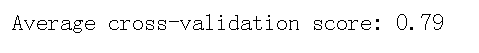
The larger the value of k, the greater the amount of calculation, which may be unbearable, so it needs to be selected carefully.

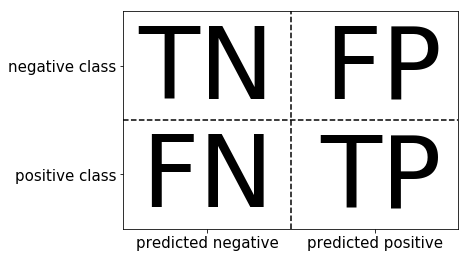
2. Confusion matrix

*TP(True Positive): predict the positive class as the number of positive classes. The true value is 1 and the predicted value is 1

*FN(False Negative): predict the number of positive classes as the number of negative classes. The true value is 1 and the predicted value is 0

*FP(False Positive): the negative class is predicted to be the number of positive classes. The true value is 0 and the predicted value is 1

*TN(True Negative): predict the negative class as the number of negative classes. The true value is 0 and the predicted value is 0

 

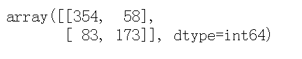
from sklearn.metrics import confusion_matrix
# Training model
lr = LogisticRegression(C=100)
lr.fit(X_train, y_train)
# Model prediction results
pred = lr.predict(X_train)
# Confusion matrix
confusion_matrix(y_train, pred)

 

from sklearn.metrics import classification_report
# Accuracy, recall and F1 score
print(classification_report(y_train, pred))

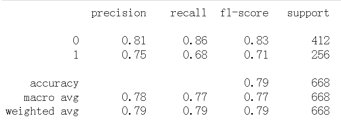
It can be seen that the accuracy of this model is 79%, in which the accurate probability of predicting death (i.e. 0) is 81%, and the accurate probability of predicting survival (i.e. 1) is 75%, indicating that the prediction effect of this model is good.

 3.ROC curve

The full name of ROC is Receiver Operating Characteristic Curve, that is, the working characteristic curve of the subject. The abscissa of the curve is false positive rate (FPR) and the ordinate is true positive rate (TPR). TPR=TP/(TP+FN),FPR=FP/(FP+TN). The larger the area surrounded under the ROC curve, the better the TPR, and the smaller the FPR, the better. The two indicators restrict each other.

from sklearn.metrics import roc_curve
fpr, tpr, thresholds = roc_curve(y_test, lr.decision_function(X_test))
plt.plot(fpr, tpr, label="ROC Curve")
plt.xlabel("FPR")
plt.ylabel("TPR (recall)")
# The threshold closest to 0 was found
close_zero = np.argmin(np.abs(thresholds))
plt.plot(fpr[close_zero], tpr[close_zero], 'o', markersize=10, label="threshold zero", fillstyle="none", c='k', mew=2)
plt.legend(loc=4)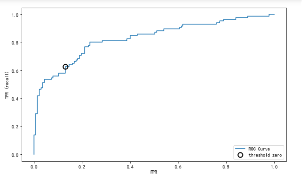

When a threshold is specified, instances greater than this threshold are classified as positive, and instances less than this value are classified as negative. Each point on the ROC curve corresponds to a threshold. For a classifier, there will be a TPR and FPR under each threshold. The closer the ROC is to the upper left corner, the better the classifier effect. Finding the threshold closest to 0 can be used to judge the effect of 0-1 classification, and the prediction model is good.

Summary: in the third chapter, I learned more about machine learning about model establishment and evaluation, and came into contact with classification model, prediction label, cross validation, confusion matrix, ROC curve and other knowledge. With more confusion, I also realized that I have a lot to learn and gained a lot.