Chapter VI fundamentals of visual processing

6.1 introduction to convolutional neural network

         The convolution neural network is composed of one or more convolution layers and the top fully connected layer (corresponding to the classical neural network), as well as the correlation weight and Pooling Layer. Figure 6-1 is a convolutional neural network architecture.

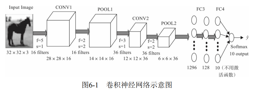
         Figure 6-1 shows the general structure of convolutional neural network, including common layers of convolutional neural network, such as convolution layer, pooling layer, full connection layer and output layer; Some also include other layers, such as regularization layer, advanced layer, etc. The convolutional neural network is defined in code.

  1) Import related modules

import torch
import torch.nn as nn
import torch.nn.functional as F
import torch.optim as optim
from torchvision import datasets, transforms

  2) Define network (for figure 6-1)

class CNNNet01(nn.Module):
    def __init__(self):
        super(CNNNet,self).__init__()
        self.conv1 = nn.Conv2d(in_channels=3,out_channels=16,kernel_size=5,stride=1)
        self.pool1 = nn.MaxPool2d(kernel_size=2,stride=2)
        self.conv2 = nn.Conv2d(in_channels=16,out_channels=36,kernel_size=5,stride=1)
        self.pool2 = nn.MaxPool2d(kernel_size=2, stride=2)
        self.dense1 = nn.Linear(900,128)
        self.dense2 = nn.Linear(128,10)
      

    def forward(self,x):
        x=self.pool1(F.relu(self.conv1(x)))
        x=self.pool2(F.relu(self.conv2(x)))
        x=x.view(-1,900)
        x=F.relu(self.dense2(F.relu(self.dense1(x))))
        return x

6.2 convolution

         Convolution layer is the core layer of convolution neural network, and convolution is the core of convolution layer.

         reference resources: Convolution and deconvolution in CNN_ HHzdh blog - CSDN blog

        reference resources: Calculation formula of convolution and deconvolution output_ HHzdh blog - CSDN blog_ Deconvolution formula

6.2.1 convolution kernel

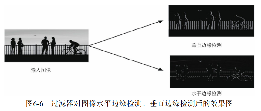
         Convolution kernel is the core of the whole convolution process. Simpler convolution kernels or filters include Horizontalfilter, Verticalfilter, Sobel Filter, etc. These filters can detect the horizontal and vertical edges of the image, enhance the weight of the central area of the image, and so on.

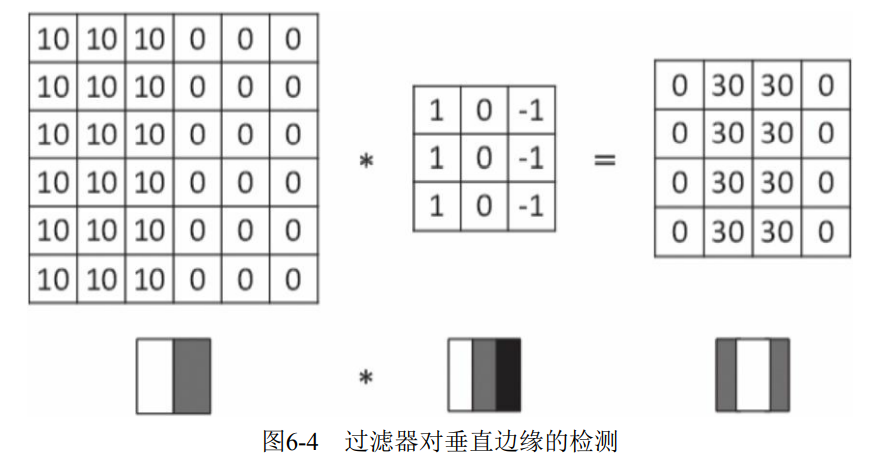
1) Vertical edge detection.

         This filter is 3 × 3 matrix (Note: the filter is generally an odd order matrix), which is characterized by the first and third columns with values, and the second column is 0. After this filter, the vertical edge of the original data is detected, as shown in Figure 6-4.

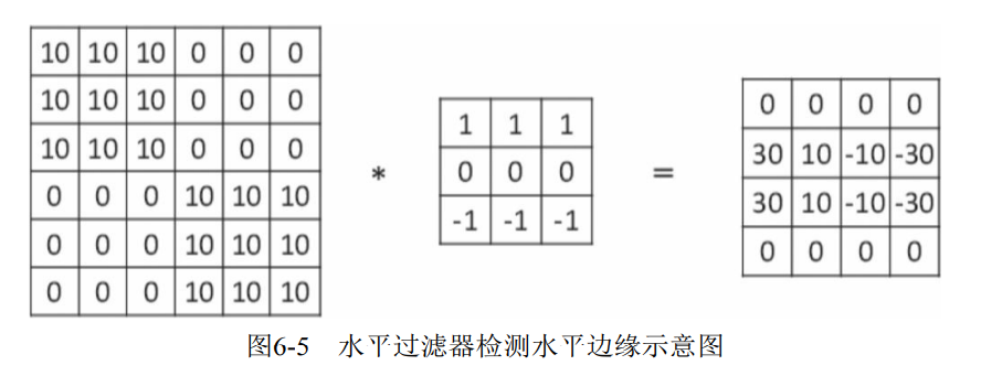
  2) Horizontal edge detection.

         three × 3 matrix, which is characterized by the first and third rows with values, and the second row is 0. After this filter, the horizontal edge of the original data is detected.

6.2.2 stride

         The number of cells each time a small window (actually a convolution kernel or filter) moves in the left window (whether from left to right or from top to bottom) is called strides, which is the number of pixels skipped in the image.

6.2.3 filling

         When the input picture does not match the convolution kernel or the convolution kernel exceeds the picture boundary, the boundary filling method can be used. That is, expand the picture size and fill the expanded area with zero, as shown in Figure 6-10. Of course, it can not be extended.

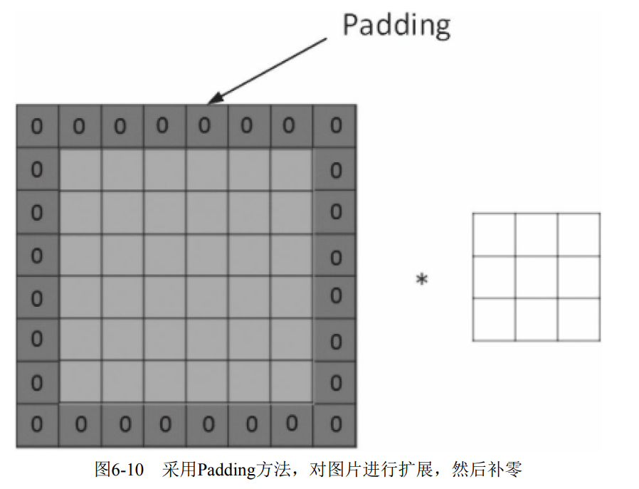
         Generally, the Same mode is selected. Using the Same mode will not lose information.

6.2.4 convolution on multiple channels  

         The convolution operation of 3-Channel pictures is basically the same as that of single Channel pictures. For 3-Channel RGB pictures, the corresponding filter operator is also 3-Channel. For example, a picture is 6 × six × 3. It represents the Height, width and Channel of the picture respectively. The process is to convolute and sum each single Channel (R, G, B) with the corresponding filter, and then add the sum of the three channels to obtain a pixel value of the output picture.

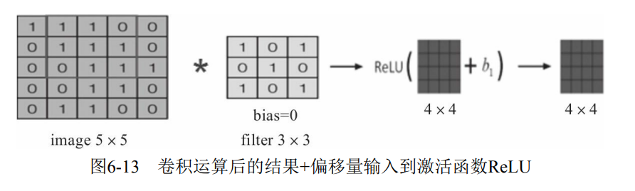
6.2.5 activation function

         The convolution neural network is similar to the standard neural network. In order to ensure its nonlinearity, the activation function also needs to be used, that is, after the convolution operation, the output value plus the offset is input to the activation function, and then used as the input of the next layer, as shown in Fig. 6-13. The commonly used activation functions are nn.Sigmoid, nn.ReLU, nnLeakyReLU, nn.Tanh, etc.

6.2.6 convolution function  

Conv2d(in_channels, out_channels, kernel_size, stride=1,padding=0, dilation=1, groups=1,bias=True, padding_mode='zeros')

          The meanings of the five common parameters are as follows:

• in_channels: enter the number of channels;
• out_channels: number of output channels;
• kernel_size: size of convolution kernel;
• Stripe: the step size of each sliding of convolution;
• Padding: padding, which sets the size of the margin with a value of 0 added to all boundaries.

         The calculation formula of convolution network: N=(W-F+2P)/S+1, where N: output size, W: input size, F: convolution kernel size, P: filling value size, s: step size

  example:

# batch norm and leaky relu functions promote healthy gradient flow
class Discriminator(nn.Module):
    def __init__(self, ngpu):
        super(Discriminator, self).__init__()
        self.ngpu = ngpu
        self.main = nn.Sequential(
            # input is (nc) x 64 x 64     128,3*64*64
            nn.Conv2d(nc, ndf, 4, 2, 1, bias=False), # 64-4+2/2+1=32  
            nn.LeakyReLU(0.2, inplace=True),
            # state size. (ndf) x 32 x 32  64*32*32
            
            nn.Conv2d(ndf, ndf * 2, 4, 2, 1, bias=False), # 32-4+2/2+1=16
            nn.BatchNorm2d(ndf * 2),
            nn.LeakyReLU(0.2, inplace=True), 
            # state size. (ndf*2) x 16 x 16  128*16*16
            
            nn.Conv2d(ndf * 2, ndf * 4, 4, 2, 1, bias=False), # 16-4+2/2+1=8
            nn.BatchNorm2d(ndf * 4), # 256
            nn.LeakyReLU(0.2, inplace=True),
            # state size. (ndf*4) x 8 x 8   256*8*8
            
            nn.Conv2d(ndf * 4, ndf * 8, 4, 2, 1, bias=False), # 8-4+2/2+1=4
            nn.BatchNorm2d(ndf * 8),
            nn.LeakyReLU(0.2, inplace=True),
            # state size. (ndf*8) x 4 x 4  512*4*4
            
            nn.Conv2d(ndf * 8, 1, 4, 1, 0, bias=False), # 4-4/2+1=1
            nn.Sigmoid() # 128,1*1024
        )

    def forward(self, input):
        return self.main(input)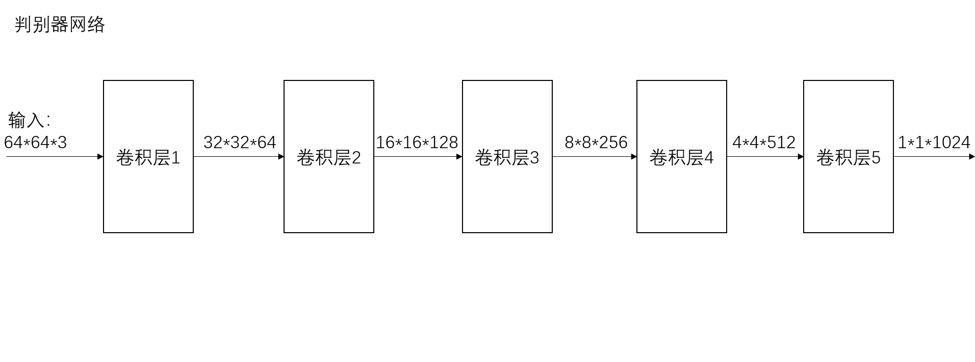

 

  Some points:

• Conv1d: for text data, only the width is convoluted, not the height, while Conv2d: for image data, both the width and height are convoluted
• Conv2d (number of input channels, number of output channels, and kernel_size). When the convolution kernel is square, write only one, but when the convolution kernel is not square, write both length and width, as follows nn.Conv2d(H,W,...)

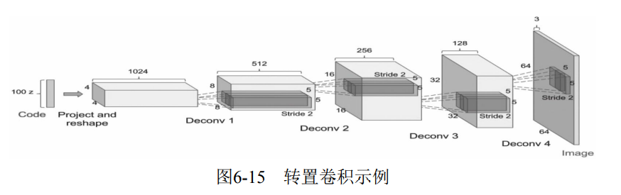
6.2.7 transpose convolution

         Transposed Convolution is also called Deconvolution or fractionally strided convolution in some literatures. Transpose convolution is widely used in Generative countermeasure network (GAN).

    The deconvolution function in pytorch is:

class torch.nn.ConvTranspose2d(in_channels, out_channels, kernel_size, stride=1, padding=0,output_padding=0,groups=1,bias=True, dilation=1)
# Generally the following
nn.ConvTranspose2d(in_channels, out_channels, kernel_size, stride, padding)

         The meaning of parameters is as follows:

• in_channels(int) – the number of channels of the input signal
• out_channels(int) – number of channels generated by convolution
• kernel_size(int or tuple) - the size of convolution kernel
• Strip (int or tuple, optional) - convolution step size, that is, the multiple to expand the input.
• Padding (int or multiple, optional) - the number of layers of 0 is added to each input edge, and the height and width are increased by 2*padding
• output_padding(int or tuple, optional) - the number of layers of 0 is added to the output edge, and the height and width are increased
• groups(int, optional) – the number of blocked connections from the input channel to the output channel
• bias(bool, optional) - if bias=True, add bias
• Division (int or tuple, optional) – the spacing between convolution kernel elements

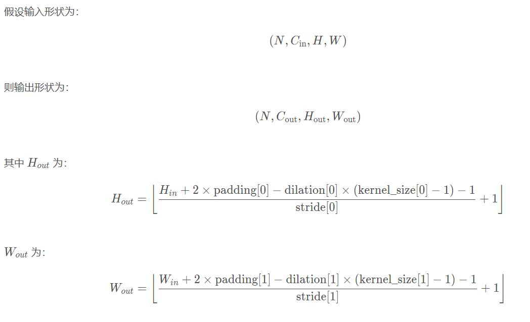
         For the calculation of input and output, first, the parameter out_channels specifies the number of output channels, that is, it must be output_size*output_size*out_channels, so it mainly calculates the output of the output_size, the formula is as follows:

        

         In general, the following formula is used:

         

  example:

# Generator Code
# Generator deconvolution
class Generator(nn.Module):
    def __init__(self, ngpu):
        super(Generator, self).__init__()
        self.ngpu = ngpu  # Number of GPUs available. Use 0 for CPU mode.
        self.main = nn.Sequential(
            # Input is Z, going into a revolution 
            nn.ConvTranspose2d( nz, ngf * 8, 4, 1, 0, bias=False), #(1-1)*1+4-2*0=4  
            nn.BatchNorm2d(ngf * 8),
            nn.ReLU(True),
            # state size. (ngf*8) x 4 x 4   4*4*512
            '''
            class torch.nn.ConvTranspose2d(in_channels, out_channels, kernel_size, stride=1, padding=0, 
                                                       output_padding=0, groups=1, bias=True, dilation=1)
            '''
            
            
            nn.ConvTranspose2d(ngf * 8, ngf * 4, 4, 2, 1, bias=False), # (4-1)*2-2*1+4=8
            nn.BatchNorm2d(ngf * 4),
            nn.ReLU(True),
            # state size. (ngf*4) x 8 x 8   8*8*256
            
            nn.ConvTranspose2d( ngf * 4, ngf * 2, 4, 2, 1, bias=False), # (8-1)*2-2*1+4=16
            nn.BatchNorm2d(ngf * 2),
            nn.ReLU(True),
            # state size. (ngf*2) x 16 x 16  16*16*128
            
            nn.ConvTranspose2d( ngf * 2, ngf, 4, 2, 1, bias=False), # (16-1)*2-2*1+4=32
            nn.BatchNorm2d(ngf),
            nn.ReLU(True),
            # state size. (ngf) x 32 x 32   32*32*64
            
            
            nn.ConvTranspose2d( ngf, nc, 4, 2, 1, bias=False), # (32-1)*2-2*1+4=64
            nn.Tanh()
            # state size. (nc) x 64 x 64   64*64*3
        )

    def forward(self, input):
        return self.main(input)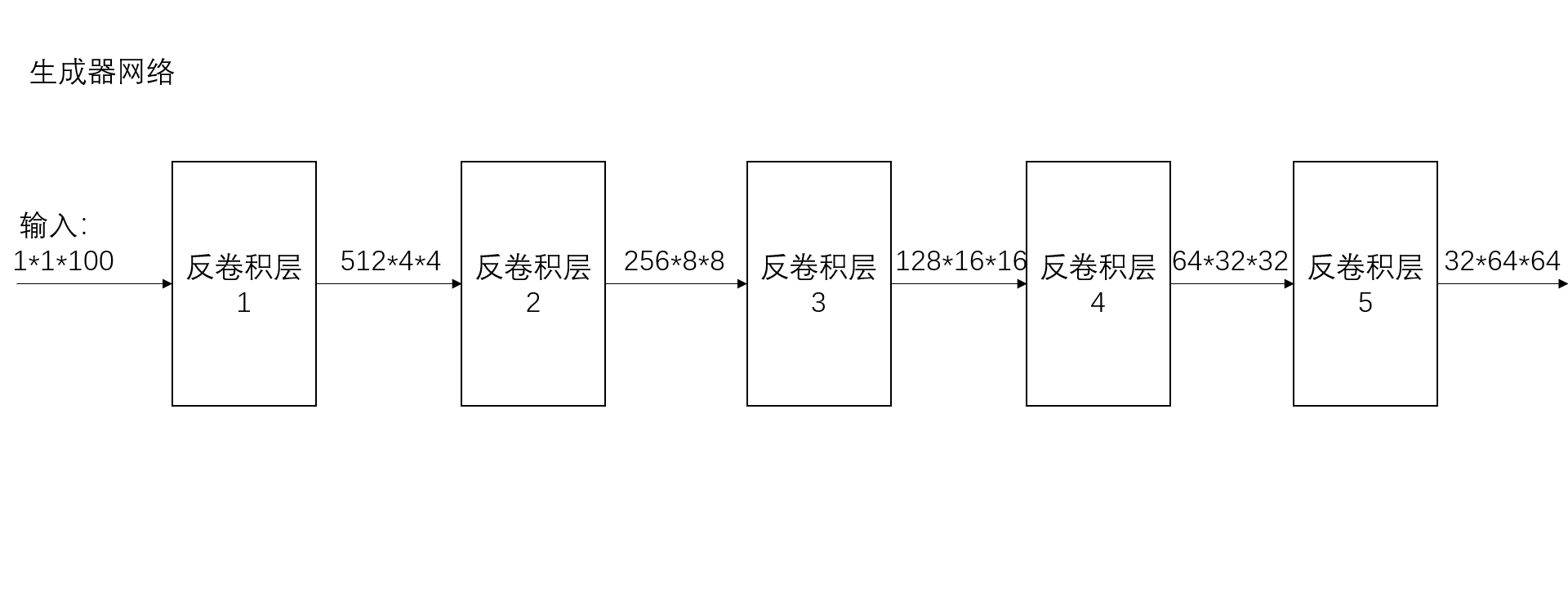

 6.3 pool layer  

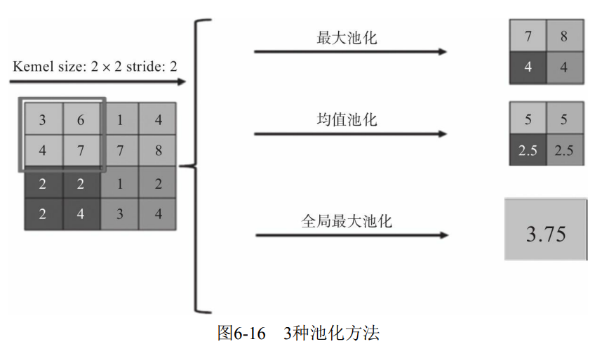
         There are three common pooling methods.

• Max Pooling: select the maximum value in the Pooling window as the sampling value.
• Mean Pooling: add all values in the Pooling window to get the average, and take the average as the sampling value.
• Global maximum (or mean) pooling: compared with the usual maximum or minimum pooling, global pooling is the pooling of the entire feature map, not within the moving window.

  6.3.1 local pooling

         The maximum or average pooling we usually use is sliding in the form of a window on the Feature Map (similar to convolution window sliding). The operation is to take the average value in the window as the result. After the operation, the Feature Map is downsampled to reduce the over fitting phenomenon. The pooling in the moving window is called local pooling.

         nn.MaxPool2d is often used for maximum pooling, and nn.AvgPool2d is used for average pooling.

6.3.2 global pooling

         Take Global Average Pooling as an example: Global Average Pooling (GAP) does not take the mean in the form of window, but takes the characteristic graph as the unit for averaging, that is, a characteristic graph outputs a value.

6.4 modern classic network

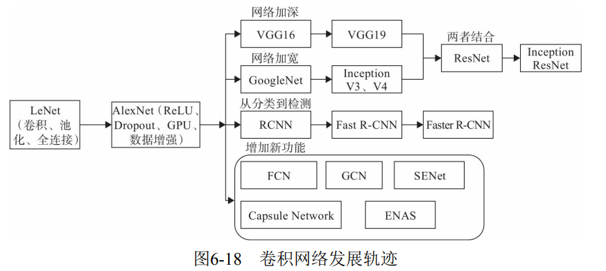
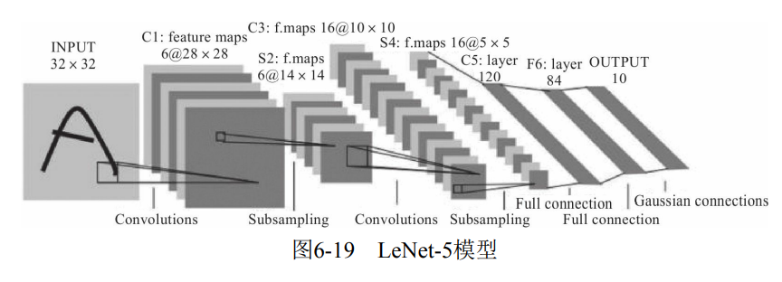
6.4.1 LeNet-5 model

(1) Model architecture LeNet-5 model structure is input layer - convolution layer - pooling layer - convolution layer - pooling layer - full connection layer - full connection layer - output, which is in series mode, as shown in Figure 6-19.

(2) Model features · each convolution layer consists of three parts: convolution, pooling and nonlinear activation function.

• Convolution is used to extract spatial features.
• The Average Pooling layer of Subsample is adopted.
• Activation function using hyperbolic tangent (Tanh).
• Finally, MLP is used as classifier.

6.4.2 Alex net model

(1) Model architecture

         AlexNet is an 8-layer deep network, including 5 layers of convolution layer and 3 layers of full connection layer, excluding LRN layer and pooling layer, as shown in Figure 6-20.

  (2) Model characteristics

• It is composed of 5-layer convolution and 3-layer full connection. The input image is 3-channel 224 × 224, and the network scale is much larger than LeNet.
• Use ReLU to activate the function.
• Dropout can be used as a regular term to prevent over fitting and improve the robustness of the model.
• Have some good training skills, including data expansion, learning rate strategy, weight delay, etc.

6.4.3 VGG model

(1) Model structure

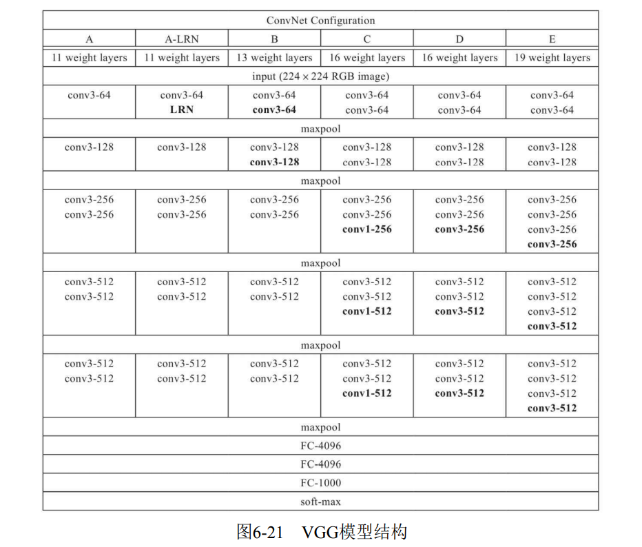
  (2) Model characteristics

• Deeper network structure: the number of network layers increased from 8 layers of AlexNet to 16 and 19 layers. A deeper network means more powerful network capability and more powerful computing power. However, later, the hardware developed rapidly and the computing power of graphics card also increased rapidly, so as to promote the rapid development of deep learning.
• Use smaller 3 × Convolution kernel of 3: 3 is used in the model × The convolution kernel of 3 because of two 3 × The receptive field of 3 is equivalent to a 5 × 5. At the same time, the number of parameters is less, and the subsequent networks basically follow this paradigm.

6.4.4 Google net model

         VGG is to increase the depth of the network, but when the depth reaches a certain level, it may become a bottleneck. GoogLeNet increases the network capacity from another dimension. Each unit has many layers of parallel computing, making the network wider. The basic units are shown in Figure 6-22.

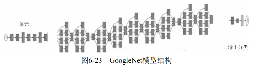
  (1) Model structure

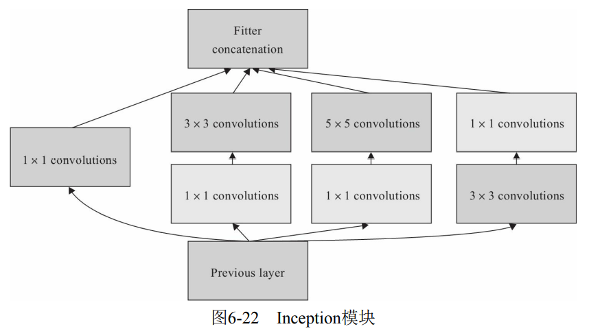
         The overall structure of the network is shown in Figure 6-23, including multiple Inception modules shown in Figure 6-22. In order to facilitate training, two auxiliary classification branches and supplementary gradients are added, as shown in Figure 6-23.

  (2) Model characteristics

• The concept structure is introduced, which is a Network In Network structure. Through the horizontal arrangement of the network, we can get better model ability with a shallow network, carry out multi feature fusion, and be easier to train at the same time. In addition, in order to reduce the amount of calculation, 1 is used × 1 convolution to reduce the dimension of the characteristic channel. Stacking Inception modules is called Inception network, and GoogLeNet is an example of well-designed Inception network (Inception v1), that is, GoogLeNet is a kind of Inception v1 network.
• Global average pooling layer is adopted. Replace all the following full connection layers with simple global average pooling, and there will be fewer parameters in the end. In AlexNet, the full connection layer parameters of the last three layers account for almost 90% of the total parameters. Using a large network allows GoogleNet to remove the full connection layer in width and depth, but it will not affect the accuracy of the results. The accuracy of 93.3% is achieved in ImageNet, which is faster than VGG. However, the problem that the network is too deep to be well trained has not been solved until ResNet proposed Residual Connection.

6.4.5 ResNet model

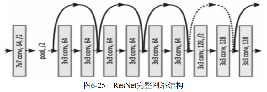
(1) Model structure

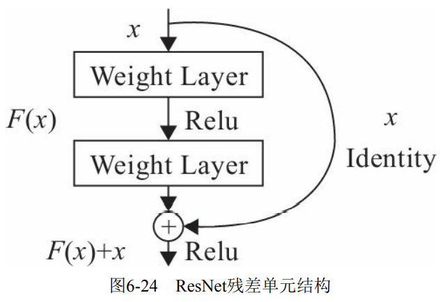
          The complete network structure is shown in Figure 6-25: by introducing residual and Identity identity mapping, it is equivalent to a gradient high-speed channel, which can be trained more easily to avoid the problem of gradient disappearance.

  (2) Model characteristics

• The number of floors is very deep, more than 100.
• The residual element is introduced to solve the degradation problem.