introduce
-
Not long ago (in fact, for a long time), the CheXNet model for CT image detection of pneumonia was reproduced with Paddle
-
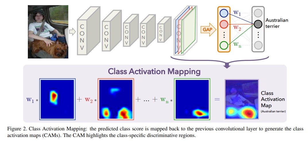
A visual method CAM is mentioned in the paper, which can visualize the activation of the network. The example is shown in the figure below:
[the external chain picture transfer fails. The source station may have an anti-theft chain mechanism. It is recommended to save the picture and upload it directly (IMG gspulcxp-1640950987901)( https://stanfordmlgroup.github.io/projects/chexnet/img/chex-main.svg )]
-
This time we will introduce how to use CAM to visualize the pneumonia detection of CT images
reference material
-
CheXNet paper: CheXNet: Radiologist-Level Pneumonia Detection on Chest X-Rays with Deep Learning
-
The padding implementation of CheXNet: jm12138/Paddle-CheXNet / Paper reproduction: Based on paddle2 0 reproduce CheXNet model
-
CAM paper: Learning Deep Features for Discriminative Localization
-
CAM reference code: zhoubolei/CAM
CAM
-
CAM, namely Class Activation Mapping, is a visual class activation algorithm, which is suitable for models containing GAP layer + softmax (sigmoid) as classification output
-
The general process is shown in the figure below:
-
The specific implementation includes the following steps:
-
Extract the output feature map of the last convolution layer
-
The weight of the classification linear layer is used to weight the feature map
-
Normalize the feature map and scale it to the input size
-
Then the characteristic map is inversely normalized to the range of 0-255
-
data set
ChestX-ray14
- ChestX-ray14 (2017) is currently the largest open source chest X-ray data set.
- It contains 112120 frontal scanning X-rays from 30805 patients and image tags of 14 categories of diseases mined from relevant radiology reports using NLP (each image can have multiple tags).
- The data set contains 14 types of common chest pathology, including atelectasis, consolidation, infiltration, pneumothorax, edema, emphysema, fibrous degeneration, effusion, pneumonia, pleural thickening, cardiac hypertrophy, nodules, masses and hernia.
Decompress dataset
- Because only some test images are needed, all data sets are not decompressed
%cd ~
!mkdir ~/dataset
!tar -xf data/data103487/images_001.tar.gz -C ~/dataset
/home/aistudio
code implementation
Synchronization code
- Download the code for paddy chexnet
!git clone https://github.com/jm12138/Paddle-CheXNet
Switch code directory
%cd ~/Paddle-CheXNet
/home/aistudio/Paddle-CheXNet
Import the necessary modules
import cv2
import numpy as np

import paddle
import paddle.nn as nn
import paddle.vision.transforms as transforms

from chexnet.densenet import DenseNet121
from chexnet.utility import N_CLASSES, CLASS_NAMES
CheXNet CAM model
-
Add CAM visualization function to the original CheXNet
-
The specific functions have been roughly mentioned earlier, and will not be repeated here. For more details, you can also refer to the paper
class CheXNetCAM(nn.Layer):
    """Model modified.

    The architecture of our model is the same as standard DenseNet121
    except the classifier layer which has an additional sigmoid function.

    """

    def __init__(self, out_size, backbone_pretrained=True):
        super(CheXNetCAM, self).__init__()
        self.out_size = out_size
        self.densenet121 = DenseNet121(pretrained=backbone_pretrained)
        num_ftrs = self.densenet121.num_features
        self.densenet121.batch_norm.register_forward_post_hook(
            self.hook_feature)
        self.densenet121.out = nn.Sequential(nn.Linear(num_ftrs, out_size),
                                             nn.Sigmoid())

    def forward(self, x):
        size = x.shape[2:]
        x = self.densenet121(x)
        cams = self.cam(self.feature, self.densenet121.out[0].weight, size)
        return x, cams

    @staticmethod
    @paddle.no_grad()
    def cam(feature_conv, weight_softmax, size):
        cams = paddle.einsum('bchw, cn -> bnhw', feature_conv, weight_softmax)
        cams = cams - paddle.min(cams, axis=[2, 3], keepdim=True)
        cams_img = cams / paddle.max(cams, axis=[2, 3], keepdim=True)
        cams_img = nn.functional.upsample(cams_img, size, mode='bilinear')
        cams_img = (255 * cams_img).cast(paddle.uint8)
        return cams_img

    def hook_feature(self, layer, input, output):
        self.feature = output
Load CheXNet CAM model
- The CAM function does not affect the original model structure, so the original pre training model can be loaded
model = CheXNetCAM(N_CLASSES, backbone_pretrained=False)
params = paddle.load('pretrained_models/model_paddle.pdparams')
model.set_dict(params)
model.eval()
data processing
net_transform = transforms.Compose([
    transforms.Resize(256),
    transforms.CenterCrop(224),
    transforms.ToTensor(),
    transforms.Normalize([0.485, 0.456, 0.406], [0.229, 0.224, 0.225]),
    lambda x:x[None, ...]
])


img_transform = transforms.Compose([
    transforms.Resize(256),
    transforms.CenterCrop(224),
    lambda x: x.astype('uint8')
])
Read input image
img_path = '/home/aistudio/dataset/images/00000001_000.png'
img = cv2.imdecode(np.fromfile(img_path, dtype=np.uint8), cv2.IMREAD_COLOR)
img_rgb = cv2.cvtColor(img, cv2.COLOR_BGR2RGB)
input_tensor = net_transform(img_rgb)
img_ori = img_transform(img)
Model forward calculation
- Calculate class scores and CAM visualization images
with paddle.no_grad():
    results, cams = [x.numpy() for x in model(input_tensor)]
Output processing
- Overlay original image and CAM visualization image
- Drawing labels is the category score
- merge images
save_path = '../cams.jpg'
img_cp = img_ori.copy()
cv2.putText(img_cp, 'Original', (5, 224-5),
            cv2.FONT_HERSHEY_SIMPLEX, 0.5, (255, 255, 255), 1)

mixes = [img_cp]
for i, cam in enumerate(cams[0]):
    heatmap = cv2.applyColorMap(cam, cv2.COLORMAP_JET)
    mix = (heatmap * 0.3 + img_ori * 0.5).astype('uint8')
    cv2.putText(mix, f'{CLASS_NAMES[i]}: {results[0][i]*100:.02f}%', (5, 224-5),
                cv2.FONT_HERSHEY_SIMPLEX, 0.5, (255, 255, 255), 1)
    mixes.append(mix)

a = np.concatenate(mixes[0:5], 1)
b = np.concatenate(mixes[5:10], 1)
c = np.concatenate(mixes[10:15], 1)
out = np.concatenate([a, b, c], 0)

concatenate(mixes[10:15], 1)
out = np.concatenate([a, b, c], 0)

cv2.imwrite(save_path, out)
True
Preview Results
-
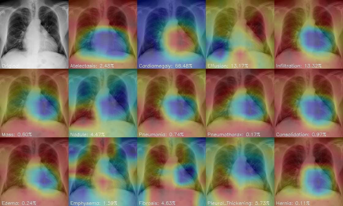
The above prediction results are shown in the figure below:
-
In the visual image, red indicates high activation intensity and blue indicates weak activation intensity
-
It can be seen that Cardiomegaly, the second category, has the highest score of cardiac hypertrophy. It can also be seen that the red part is concentrated in the chest and heart, indicating that this model can also better focus on the parts related to the disease
summary
-
A simple visualization method of model activation is introduced
-
Through such visualization, we can explain the function of the model, or find the problems in the model to further improve the model
-
Of course, cam is only a relatively simple scheme, and there are many other better improvement methods such as grad CAM / grad cam + +
-
Let's continue the introduction later