An example of image processing using DCT (discrete cosine) transform was introduced in the previous document:

Application of DCT/IDCT transform in image compression_ The vast majority of images in tugouxp's column CSDN blog have a common feature. Flat areas and areas with slow content change account for most of an image, while detail areas and content mutation areas account for a small part. It can also be said that in the image, DC and low-frequency areas account for the majority, and high-frequency areas account for a small parthttps://blog.csdn.net/tugouxp/article/details/117585190 This paper introduces the code demonstration of image processing with discrete Fourier transform.

Methods and ideas:

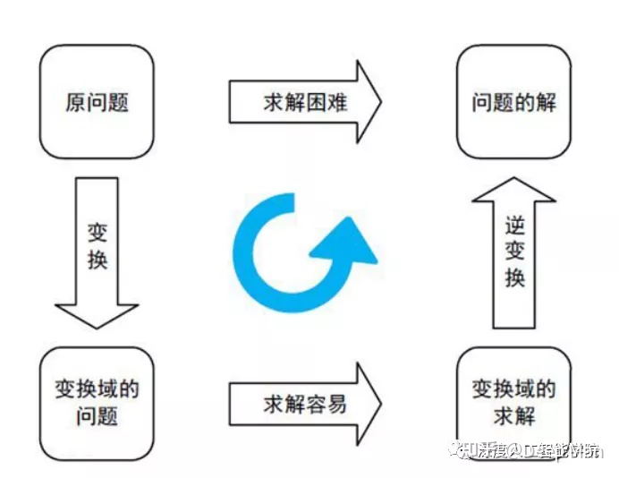
  For the practice of Fourier transform, please refer to this article:

Graph theory fourier transform_ tugouxp's column - CSDN blog_ fourier transform is like the well-known Taylor serieshttps://blog.csdn.net/tugouxp/article/details/113485640 Fourier transform is to decompose a signal curve into several sinusoidal curves. These sinusoidal frequencies represent the frequency changes of the original signal curve. In general, it is to classify the signals with different frequencies on the original signal curve. The signals at the same frequency are divided into one sinusoidal curve, so there are several sinusoidal curves with different frequencies, Some of these sinusoids are the information we need and some are unnecessary information. We can filter out the unimportant information to get the information we want.

Code demonstration:

High frequency filtering operation:

#-*- coding:utf-8 -*-
import numpy
import cv2
import matplotlib.pyplot as plt
import os

print (os.getcwd())#Get current directory
print (os.path.abspath('.'))#Get current working directory
 
#DFT: discrete Fourier transform '
# 2. DFT(Discrete Fourier Transform) in opencv
img = cv2.imread("./3.jpg")
# 0. Convert to grayscale image
gray = cv2.cvtColor(img, cv2.COLOR_BGR2GRAY)
rows, cols = gray.shape
 
# 1.DFT discrete Fourier transform: spatial - > frequency domain
dft = cv2.dft(src=numpy.float32(gray), flags=cv2.DFT_COMPLEX_OUTPUT)  # src is a grayscale image and is of type numpy.float32
print(dft.shape)#Two channels
 
# 2. Centralization: move the low frequency to the center of the image
fftshift = numpy.fft.fftshift(dft)
# Obtain amplitude spectrum (for displaying pictures): numpy.log () is to limit the value to [0255]
magnitude_spectrum = numpy.log(cv2.magnitude(fftshift[:, :, 0], fftshift[:, :, 1]))
 
# 3. Low pass filtering of filtering operation (removing high frequency and maintaining low frequency)
mask = numpy.zeros((rows, cols,2), dtype=numpy.uint8)
mask[(rows // 2 - 30): (rows // 2 + 30), (cols // 2 - 30): (cols // 2 + 30)] = 1
fftshift = fftshift * mask
 
# 4. Decentralization: restore the position of low frequency and high frequency
ifftshift = numpy.fft.ifftshift(fftshift)
 
# 5. Inverse Fourier transform: frequency domain - > spatial domain
idft = cv2.idft(ifftshift)
 
# 6. Two dimensional vector modulus (amplitude)
img_back = cv2.magnitude(idft[:, :, 0], idft[:, :, 1])
 
# Display multiple pictures in combination with matplotlib
plt.figure(figsize=(10, 10))
plt.subplot(221), plt.imshow(gray, cmap="gray"), plt.title("Input Gray Image")
plt.xticks([]), plt.yticks([])
plt.subplot(222), plt.imshow(magnitude_spectrum, cmap="gray"), plt.title("Magnitude Spectrum")
plt.xticks([]), plt.yticks([])
plt.subplot(223), plt.imshow(img_back, cmap="gray"), plt.title("Image after LPF")
plt.xticks([]), plt.yticks([])
plt.subplot(224), plt.imshow(img_back), plt.title("Result in JET")  # Default cmap='jet '
plt.xticks([]), plt.yticks([])
plt.show()

  Operation effect:

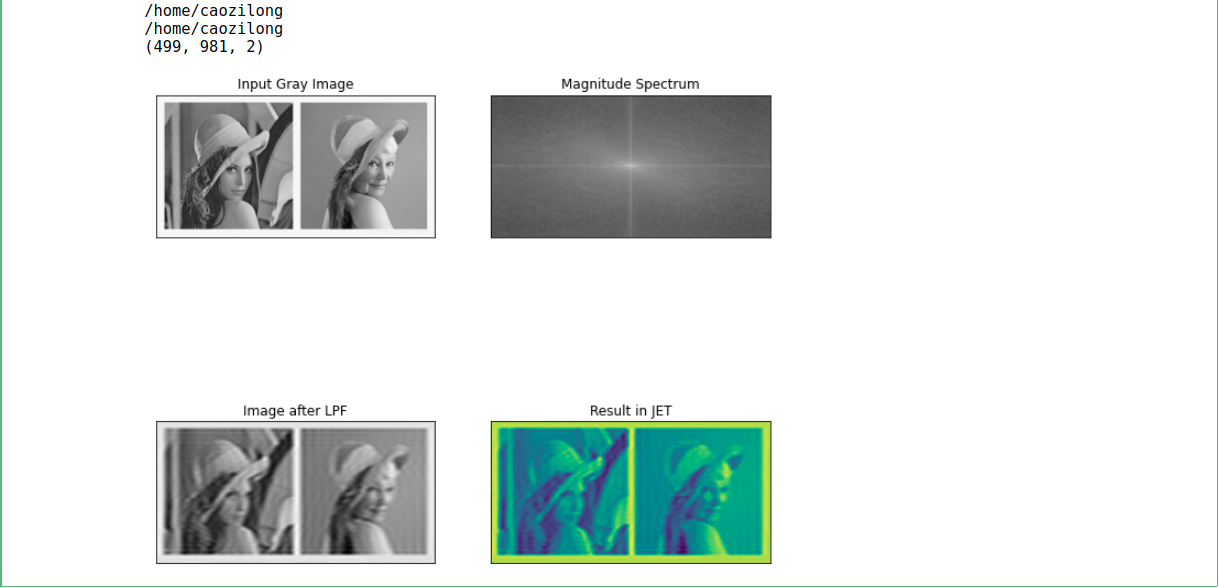
Through the above case, we intuitively feel the actual effect of Fourier transform in image denoising. After removing the high-frequency signal, whether it is the gray image or the default color image, the image contour will be softened and the boundary will become blurred. This is because the noise and edge parts of the image often change greatly, and the places with large gradient belong to high-frequency signals, Therefore, it will soften the image edge while denoising.

Next, we perform a reverse operation, that is, image high pass filtering, that is, remove the low-frequency signal and leave the high-frequency signal to see what changes the processed image will eventually have. This time, we take the fast Fourier transform in numpy as an example to realize the image high pass filtering operation:

import numpy
import cv2
import matplotlib.pyplot as plt
import os
 
img = cv2.imread("./3.jpg")
# 0. Convert to grayscale image
gray = cv2.cvtColor(img, cv2.COLOR_BGR2GRAY)
rows, cols = gray.shape
print(gray.shape)
 
# 1.FFT fast Fourier transform: spatial - > frequency domain
fft = numpy.fft.fft2(gray)  # Fourier transform, the parameter is gray image
print(fft.shape)
 
# 2. Centralization: move the low-frequency signal to the image center
fftshift = numpy.fft.fftshift(fft)
print(numpy.min(numpy.abs(fftshift)))#Absolute minimum frequency signal
print(numpy.max(fftshift),numpy.min(fftshift))#Highest frequency signal
# Obtain amplitude spectrum (for displaying pictures): numpy.log () is used to compress the value near [0255]
magnitude_spectrum = numpy.log(numpy.abs(fftshift))
print(numpy.max(magnitude_spectrum),numpy.min(magnitude_spectrum))
 
# 3. High pass filtering of filtering operation (removing low frequency and maintaining high frequency)
fftshift[rows // 2 - 50:rows // 2 + 50, cols // 2 - 50: cols // 2 + 50] = 0
# print(fftshift.shape)
 
# 4. Decentralization: restore the remaining low-frequency and high-frequency positions
ifftshift = numpy.fft.ifftshift(fftshift)
 
# 5. Inverse Fourier transform: frequency domain - > spatial domain
ifft = numpy.fft.ifft2(ifftshift)
# print(ifft)
 
# 6. Two dimensional vector modulus (amplitude)
img_back = numpy.abs(ifft)
 
#Display multiple pictures in combination with matplotlib
plt.figure(figsize=(10, 10))
plt.subplot(221), plt.imshow(gray, cmap="gray"), plt.title("Input Gray Image")
plt.xticks([]), plt.yticks([])
plt.subplot(222), plt.imshow(magnitude_spectrum, cmap="gray"), plt.title("Magnitude Spectrum")
plt.xticks([]), plt.yticks([])
plt.subplot(223), plt.imshow(img_back, cmap="gray"), plt.title("Image after HPF")
plt.xticks([]), plt.yticks([])
plt.subplot(224), plt.imshow(img_back), plt.title("Result in JET")  # Default cmap='jet '
plt.xticks([]), plt.yticks([])
plt.show()

Operation effect:

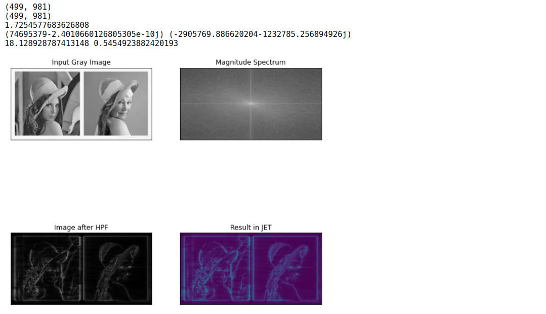
The effect of image high pass filtering is just opposite to that of low-pass filtering. From the results of the above case, the operation of high pass filtering will make the image lose more background details and only retain the corresponding contour interface of the image. This is because the image gradient change of the background part is smaller than that of the contour part. The part with small image gradient change belongs to low-frequency signal. Removing this part of low-frequency signal will make the image lack transition and the edge appear stiff. When too many low-frequency signals are removed, the image will even become an edge contour.

Since we can perform high pass filtering or low-pass filtering on the image through Fourier transform, we can also perform filtering on the image with any specified frequency band. For example, medium pass filtering is to retain the data of the specified frequency band in the middle of the image and remove the high-frequency data and low-frequency data, while block filtering is to remove the data of the specified frequency band in the middle of the image, Retain high and low frequency data.

end!