1, Recommended model construction process
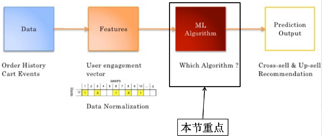
Data - > features - > ML algorithm - > prediction output
1.1 data cleaning / data processing

data sources
- Dominant data
- Rating
- Comments / comments
- Invisible data
- Order history
- Cart events plus shopping cart
- Page views page browsing
- Click thru Click
- Search log search record
Data volume / whether the data can meet the requirements
1.2 characteristic Engineering

Filter features from data
- A given product may be purchased by users with similar tastes or needs
- Use user behavior data to describe products

Representing features with data
-
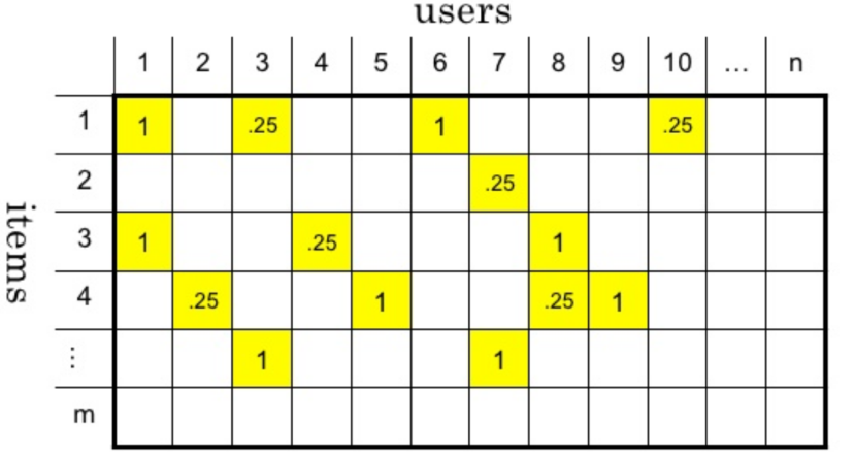
Combine all user behaviors to form a user item matrix
1.3 select the appropriate algorithm
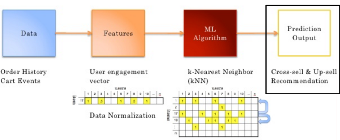
1.4 generate recommendation results
2, Collaborative Filtering recommendation algorithm
Algorithmic idea: birds of a feather flock together
The basic collaborative filtering recommendation algorithm is based on the following assumptions:
- "You are likely to like things that people like similar to you like": user based collaborative filtering recommendation (CF)
- "You are likely to like something similar to what you like": item based collaborative filtering recommendation (CF)
There are several steps to implement collaborative filtering recommendation:
-
Find the most similar person or item: TOP-N similar person or item
By calculating the similarity of two pairs to sort, we can find out the people or items similar to TOP-N
-
Generate recommendation results based on similar people or items
Use the TOP-N results to generate the initial recommendation results, and then filter out the items that the user has recorded or clearly expressed no interest
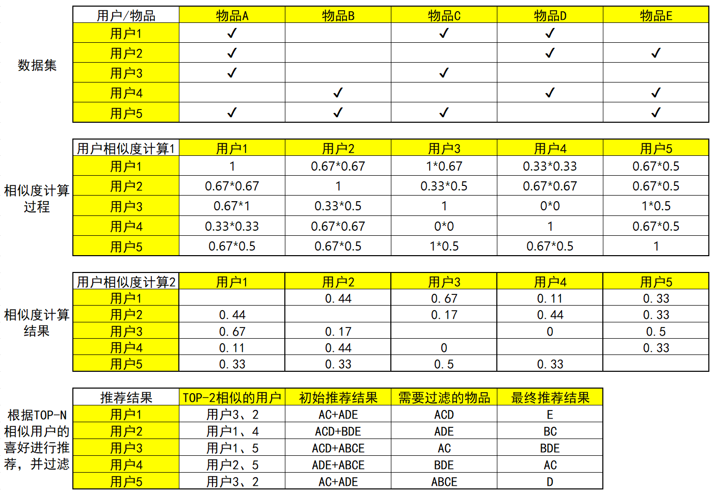
The following is a simple example. The data set is equivalent to a user's purchase record table of items: a tick indicates that the user has a purchase record of items
For similarity calculation, let's first use a simple idea: if there are two students X and y, X likes [football, basketball and table tennis] and Y likes [tennis, football, basketball and badminton], it can be seen that they have two common hobbies, so their similarity can be expressed by: 2 / 3 * 2 / 4 = 1 / 3 ≈ 0.33.
2.1 User-Based CF
2.2 Item-Based CF

Through the previous two demo s, I believe you should have a clear understanding of the design and implementation of collaborative filtering recommendation algorithm.
3, Similarity calculation

3.1 calculation method of similarity
data classification
- Real value (item scoring)
- Boolean value (whether the user's behavior is favorite or not)
Euclidean distance
Euclidean distance is a measure of distance in Euclidean space Two objects are represented as two points in the same space. If they are called P and Q, they are n coordinates respectively, then the Euclidean distance is to measure the distance between the two points Euclidean distance does not apply between Boolean vectors
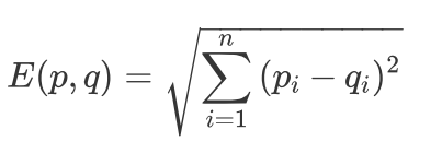
The value of Euclidean distance is a non negative number, and the maximum value is positive and infinite. Generally, the result of calculating similarity is expected to be between [- 1,1] or [0,1], which can be used generally
The following conversion formula: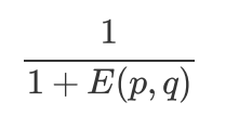
Jacquard similarity & cosine similarity & Pearson correlation coefficient
- cosine similarity
- It measures the angle between two vectors, and uses the cosine of the angle to measure similar situations
- When the angle between two vectors is 0, the cosine value is 1. When the angle is 90 degrees, the cosine value is 0 and 180 degrees, the cosine value is - 1
- Cosine similarity is commonly used to measure text similarity, user similarity and item similarity
- The characteristic of cosine similarity has nothing to do with the vector length. The calculation of cosine similarity should normalize the vector length. As long as the two vectors have the same direction, they can be regarded as' similar 'regardless of the degree
- Pearson correlation coefficient
- In fact, it is also a kind of cosine similarity, but first centralize the vector, subtract the mean value of vector a and B respectively, and then calculate the cosine similarity
- Pearson similarity calculation results are between - 1 and 1, - 1 indicates negative correlation and 1 indicates positive correlation
- Measure whether two variables increase and decrease at the same time
- Pearson correlation coefficient measures whether the change trends of the two variables are consistent, which is not suitable for calculating the correlation between Boolean vectors
- Jaccard
- The proportion of the number of intersection elements of two sets in the union set is very suitable for Boolean vector representation
- A molecule is a dot product of two Boolean vectors, and the result is the number of intersection elements
- Denominator is the sum of two Boolean vectors
- Cosine similarity is suitable for user rating data (real value), and jackard similarity is suitable for implicit feedback data (0,1 Boolean value) (collect, click, add shopping cart)
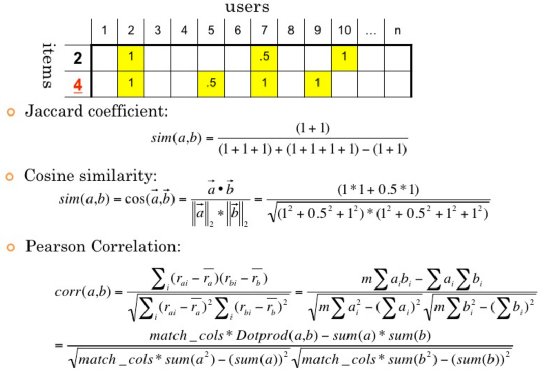
-
cosine similarity
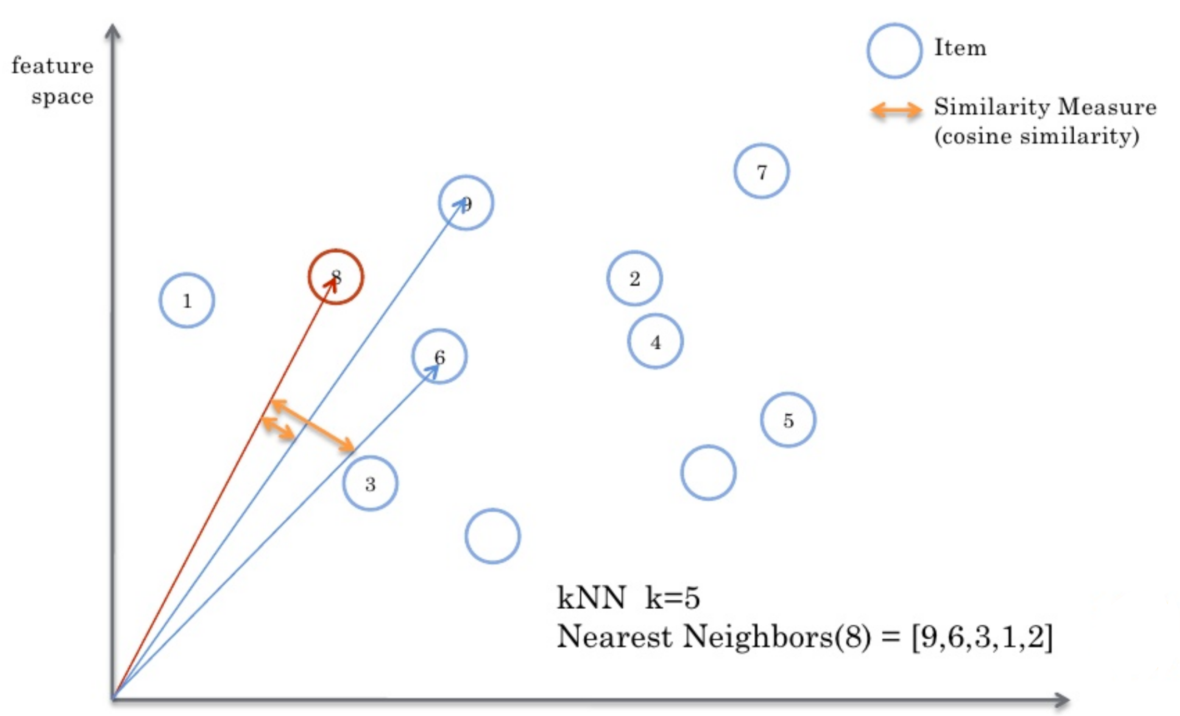
-
Pearson correlation coefficient
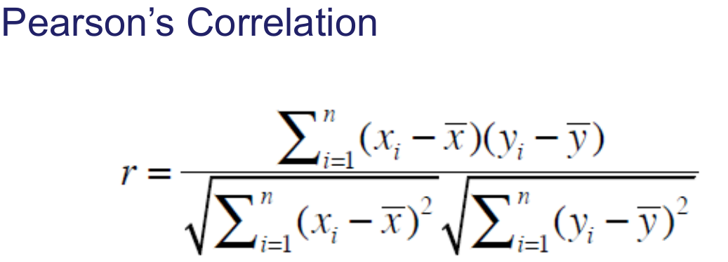
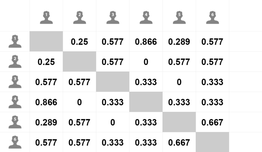
3.2 user similarity calculation
- Calculate the similarity between user 1 and other users
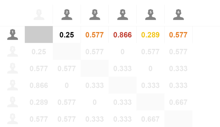
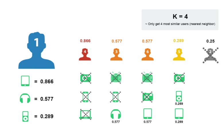
- Sort according to the similarity, k nearest neighbor, such as K, takes 4:

- Take out the shopping list of nearby users
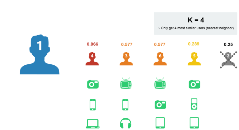
- Remove the goods that user 1 has purchased
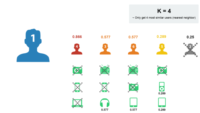
- Sort the remaining items according to the score
3.3 item similarity calculation
- Cosine similarity is not sensitive to the absolute value
- User A scored the two movies 1 and 2 respectively. User B scored the same two movies 4 and 5 respectively. The similarity between the two users was 0.98 calculated by cosine similarity
- The improved cosine similarity can be used. First calculate the mean value of each dimension of the vector, and then subtract the mean value of each vector in each dimension to calculate the cosine similarity. The similarity calculated with the adjusted cosine similarity is -0.1
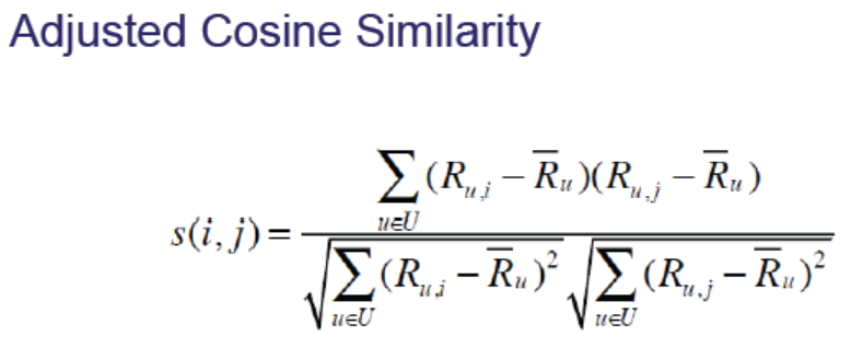
- Item similarity calculation case
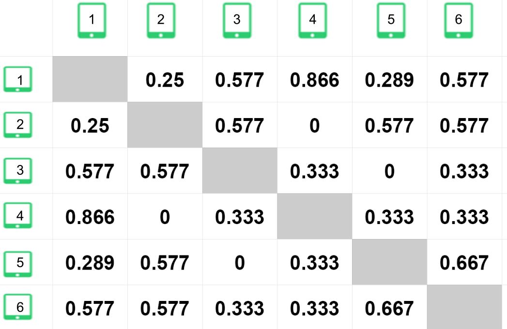
- Find similar items of item 1
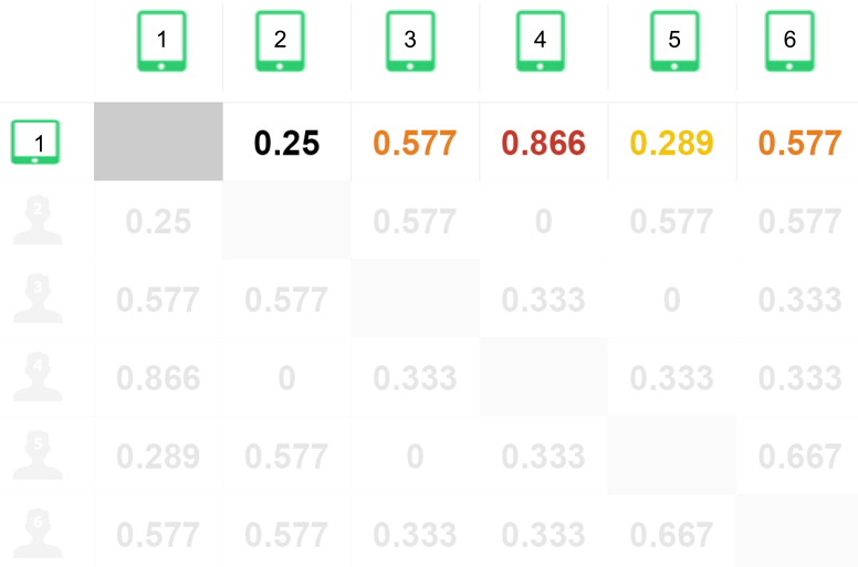
- Select the nearest item

4, Code implementation of collaborative filtering recommendation algorithm
4.1 building data sets
During calculation, we usually need to process or encode the data in order to facilitate our calculation and processing of the data. For example, here is a relatively simple case. We use 1 and 0 respectively to indicate whether the user has purchased the item. Then our data set is as follows:
import pandas as pd
users = ["User1", "User2", "User3", "User4", "User5"]
items = ["Item A", "Item B", "Item C", "Item D", "Item E"]
# User purchase record data set
datasets = [
    [1,0,1,1,0],
    [1,0,0,1,1],
    [1,0,1,0,0],
    [0,1,0,1,1],
    [1,1,1,0,1],
]
df = pd.DataFrame(datasets,columns=items,index=users)
print(df)
  Item A  Item B  Item C  Item D  Item E
User1       1       0       1       1       0
User2       1       0       0       1       1
User3       1       0       1       0       0
User4       0       1       0       1       1
User5       1       1       1       0       1
4.2 similarity calculation
With the data set, we can calculate the similarity, but there are many special similarity calculation methods, such as cosine similarity, Pearson correlation coefficient, jackard similarity and so on. Here we choose to use the jacquard similarity coefficient [0,1]
# Directly calculate the jackard similarity coefficient of some two terms
from sklearn.metrics import jaccard_score
# Calculate the similarity between Item A and Item B
print(jaccard_score(df["Item A"], df["Item B"]))
0.2
# Calculate the jackard similarity coefficient of all data
# pairwise_distance refers to calculating the distance between the corresponding elements of two input matrices X and Y
from sklearn.metrics.pairwise import pairwise_distances
# Calculate the similarity between users
user_similar = 1 - pairwise_distances(df.values, metric="jaccard")
user_similar = pd.DataFrame(user_similar, columns=users, index=users)
print("Pairwise similarity between users:")
print(user_similar)
Pairwise similarity between users:
          User1  User2     User3  User4  User5
User1  1.000000   0.50  0.666667    0.2    0.4
User2  0.500000   1.00  0.250000    0.5    0.4
User3  0.666667   0.25  1.000000    0.0    0.5
User4  0.200000   0.50  0.000000    1.0    0.4
User5  0.400000   0.40  0.500000    0.4    1.0
# Calculate the similarity between items
item_similar = 1 - pairwise_distances(df.values.T, metric="jaccard")
item_similar = pd.DataFrame(item_similar, columns=items, index=items)
print("Pairwise similarity between items:")
print(item_similar)
Pairwise similarity between items:
        Item A    Item B  Item C  Item D    Item E
Item A    1.00  0.200000    0.75    0.40  0.400000
Item B    0.20  1.000000    0.25    0.25  0.666667
Item C    0.75  0.250000    1.00    0.20  0.200000
Item D    0.40  0.250000    0.20    1.00  0.500000
Item E    0.40  0.666667    0.20    0.50  1.000000
With pairwise similarity, we can then screen the TOP-N similarity results and recommend them
4.3 User-Based CF
import pandas as pd
import numpy as np
from pprint import pprint

topN_users = {}
# Traverse each row of data
for i in user_similar.index:
    # Take out each column of data, delete itself, and then sort the data
    _df = user_similar.loc[i].drop([i])
    _df_sorted = _df.sort_values(ascending=False)

    top2 = list(_df_sorted.index[:2])
    topN_users[i] = top2

print("Top2 Similar users:")
pprint(topN_users)

rs_results = {}
# Build recommendation results
for user, sim_users in topN_users.items():
    rs_result = set()    # Store recommendation results
    for sim_user in sim_users:
        # Build initial recommendation results
        rs_result = rs_result.union(set(df.loc[sim_user].replace(0,np.nan).dropna().index))
    # Filter out purchased items
    rs_result -= set(df.loc[user].replace(0,np.nan).dropna().index)
    rs_results[user] = rs_result
print("Final recommendation result:")
pprint(rs_results)
Top2 Similar users:
{'User1': ['User3', 'User2'],
 'User2': ['User1', 'User4'],
 'User3': ['User1', 'User5'],
 'User4': ['User2', 'User5'],
 'User5': ['User3', 'User1']}
Final recommendation result:
{'User1': {'Item E'},
 'User2': {'Item C', 'Item B'},
 'User3': {'Item E', 'Item D', 'Item B'},
 'User4': {'Item C', 'Item A'},
 'User5': {'Item D'}}
4.4 Item-Based CF
import pandas as pd
import numpy as np
from pprint import pprint

topN_items = {}
# Traverse each row of data
for i in item_similar.index:
    # Take out each column of data, delete itself, and then sort the data
    _df = item_similar.loc[i].drop([i])
    _df_sorted = _df.sort_values(ascending=False)

    top2 = list(_df_sorted.index[:2])
    topN_items[i] = top2

print("Top2 Similar items:")
pprint(topN_items)

rs_results = {}
# Build recommendation results
for user in df.index:    # Traverse all users
    rs_result = set()
    for item in df.loc[user].replace(0,np.nan).dropna().index:   # Take out the current shopping list of each user
        # Find the most similar TOP-N items according to each item and build the initial recommendation result
        rs_result = rs_result.union(topN_items[item])
    # Filter out items purchased by users
    rs_result -= set(df.loc[user].replace(0,np.nan).dropna().index)
    # Add to results
    rs_results[user] = rs_result

print("Final recommendation result:")
pprint(rs_results)
Top2 Similar items:
{'Item A': ['Item C', 'Item D'],
 'Item B': ['Item E', 'Item C'],
 'Item C': ['Item A', 'Item B'],
 'Item D': ['Item E', 'Item A'],
 'Item E': ['Item B', 'Item D']}
Final recommendation result:
{'User1': {'Item E', 'Item B'},
 'User2': {'Item C', 'Item B'},
 'User3': {'Item D', 'Item B'},
 'User4': {'Item A', 'Item C'},
 'User5': {'Item D'}}
4.5 others
On the data set used by collaborative filtering recommendation algorithm
In the previous demo, we only use a purchase record of the user's items. Similarly, we can also use browsing click records, listening records and so on. In fact, the result of our prediction is equivalent to predicting whether users are interested in an item, and we can't predict the degree of preference very well.
Therefore, in the collaborative filtering recommendation algorithm, we will actually make more use of the user's "rating" data of items to predict. Through the rating data set, we can predict the user's rating of items he has not rated. The implementation principle and idea are the same as, except that the data set used is the user item scoring data.
About user item scoring matrix
There are different solutions for the user item scoring matrix according to the sparsity of the scoring matrix
-
Dense scoring matrix

-
Sparse scoring matrix

Here we first introduce the processing of dense scoring matrix. The processing of sparse matrix will be relatively complex. We will introduce it later.
5, Collaborative filtering recommendation algorithm predicts users' scores
5.1 building data sets
Objective: to predict the score of user 1 on item E
Note that when constructing score data here, we need to keep the missing part as None. If it is set to 0, it will be treated as a score value of 0
users = ["User1", "User2", "User3", "User4", "User5"]
items = ["Item A", "Item B", "Item C", "Item D", "Item E"]
# User purchase record data set
datasets = [
    [5,3,4,4,None],
    [3,1,2,3,3],
    [4,3,4,3,5],
    [3,3,1,5,4],
    [1,5,5,2,1],
]
5.2 calculating similarity
For the score data, we use Pearson correlation coefficient [- 1,1] to calculate, - 1 indicates strong negative correlation and + 1 indicates strong positive correlation
The corr method in pandas can be directly used to calculate the Pearson correlation coefficient
df = pd.DataFrame(datasets,columns=items,index=users)

print("Pairwise similarity between users:")
# Direct calculation of Pearson correlation coefficient
# By default, it is calculated by column. Therefore, if the similarity between users is calculated, it needs to be transposed
user_similar = df.T.corr()
print(user_similar.round(4))

print("Pairwise similarity between items:")
item_similar = df.corr()
print(item_similar.round(4))
Operation results:
Pairwise similarity between users:
        User1   User2   User3   User4   User5
User1  1.0000  0.8528  0.7071  0.0000 -0.7921
User2  0.8528  1.0000  0.4677  0.4900 -0.9001
User3  0.7071  0.4677  1.0000 -0.1612 -0.4666
User4  0.0000  0.4900 -0.1612  1.0000 -0.6415
User5 -0.7921 -0.9001 -0.4666 -0.6415  1.0000
 Pairwise similarity between items:
        Item A  Item B  Item C  Item D  Item E
Item A  1.0000 -0.4767 -0.1231  0.5322  0.9695
Item B -0.4767  1.0000  0.6455 -0.3101 -0.4781
Item C -0.1231  0.6455  1.0000 -0.7206 -0.4276
Item D  0.5322 -0.3101 -0.7206  1.0000  0.5817
Item E  0.9695 -0.4781 -0.4276  0.5817  1.0000
It can be seen that the most similar to user 1 are user 2 and user 3; The items most similar to item A are item E and item D, respectively.
Note: when we predict the score, we often predict through users or items with positive correlation. If there is no positive correlation, we will not be able to make prediction. This is especially common in the sparse scoring matrix, because it is difficult to obtain the positive correlation coefficient in the sparse scoring matrix.
5.3 score prediction
User based CF score prediction: use the similarity between users for prediction
There are also many schemes for score prediction. The following introduces a scheme with good effect, which considers the user's own score and the weighted average similarity score of adjacent users to predict:
If we want to predict the score of user 1 on item E, we can predict it according to user 2 and user 3 nearest to user 1. The calculation is as follows:
The similarity between user 1 and user 2 is 0.85, the similarity between user 1 and user 3 is 0.71, the score of user 2 on item E is 3, and the score of user 3 on item E is 5
Finally, it is predicted that the score of user 1 on item 5 is 3.91
Item based CF score prediction: use the similarity between items for prediction
Here, the calculation of similarity prediction of items is the same as above. The average scoring factors of users are also considered, and the prediction is carried out in combination with the weighted average similarity scoring of predicted items and similar items
If we want to predict the score of user 1 on item E, we can predict it according to item A and item D nearest to item E, which are calculated as follows:
It can be seen from the comparison that there are also differences between the user based CF prediction score and the item based CF score, because strictly speaking, they should belong to two different recommendation algorithms, which will be better than the other in different fields and scenarios, but which is better must be evaluated reasonably, Therefore, when implementing the recommendation system, these two algorithms often need to be implemented, and then evaluate and analyze the recommendation effect to select the better scheme.
6, Model based approach
6.1 ideas
-
Through the machine learning algorithm, find the pattern in the data, and model the interaction between users and items
-
The model-based collaborative filtering method is to build a more advanced algorithm of collaborative filtering
-
The problem of nearest neighbor model
- There is correlation between items, and the amount of information does not increase linearly with the increase of vector dimension
- The matrix elements are sparse, the calculation results are unstable, and a vector dimension is increased or decreased, resulting in great differences in the nearest neighbor results
6.2 algorithm classification
Graph based model
Neighborhood based models are seen as simple forms of graph based models
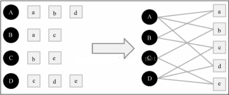
principle
- The user's behavior data is represented as a bipartite graph
- Recommendation for users based on bipartite graph
- The correlation between two vertices is evaluated according to the number of paths between two vertices, path length and the number of vertices
Model based on matrix decomposition
principle
-
Based on the potential performance of users and items, we can predict users' preference for non rated items
-
The original large matrix is approximately decomposed into the product of two small matrices. In the actual recommended calculation, the large matrix is no longer used, but the two small matrices obtained by decomposition are used
-
The user item scoring matrix A is M X N-dimensional, that is, there are M users and n items. We choose a small number k (k < < M, K < < n)
-
Two matrices u and V are obtained by calculation. U is the M * K matrix and V is the N * K matrix
\(U {m * k} V ^ {t} {n * k} is approximately equal to a {m * n} \)
The calculation process like this is matrix decomposition
6.3 method based on matrix decomposition
ALS alternating least squares
Als-wr (weighted regularized alternating least squares): alternating least squares with weighted- λ – regularization
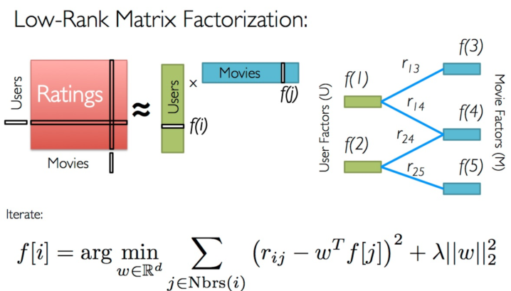
- The matrix decomposition algorithm of ALS is often used in recommendation systems. It decomposes the user's scoring matrix of items into the user's preference matrix for the implicit features of goods and the mapping matrix of goods on the implicit features. In the process of matrix decomposition, the missing items of the score are filled in, that is to say, we can recommend products to users based on the filled score.
- It is different from the traditional matrix decomposition SVD method to decompose the matrix R(R ∈ m) × n) The difference is that ALS (alternative least squares) wants to find two low dimensional matrices to R ̃ = XY to approximate matrix R, where X ∈ M × d,Y∈ℝd × n. In this way, the complexity of the problem is transformed from O(mn) to O((m+n)d).
- Process of calculating X and Y: first initialize y with a random number less than 1 and calculate x according to the formula. At this time, the initial XY matrix can be obtained. Recalculate and cover y according to the X obtained from the sum of square differences, calculate the sum of square differences, and repeat the above two steps until the sum of square differences is less than a preset number, or the iteration times meet the requirements