Authors: Chen Yingxiang, Yang Zihan

Compilation: AI Youdao

After data preprocessing, we generate a large number of new variables (for example, single hot coding generates a large number of variables containing only 0 or 1). But in fact, some newly generated variables may be redundant: on the one hand, they do not necessarily contain useful information, so they can not improve the performance of the model; On the other hand, these redundant variables will consume a lot of memory and computing power when building the model. Therefore, we should select features and select feature subsets for modeling.

Project address:

https://github.com/YC-Coder-Chen/feature-engineering-handbook

This paper will introduce the first algorithm of Feature Engineering: Filter Methods (Part 2).

catalog:

1.1.1.5 Mutual Information (regression problem)

Mutual Information measures the interdependence between variables. Its essence is entropy difference, i.e???? (????) −???? (????|????)， That is, the reduction of confusion after knowing the information of another variable. Mi is equal to zero if and only if two random variables are independent. The higher the MI value, the stronger the correlation between the two variables. Compared with Pearson correlation and F statistics, it also captures nonlinear relationships.

Formula:

• If both variables are discrete:

p(????,????) (????,????) Is the joint probability mass function (PMF) of x and y, P???? (????) Is the joint probability mass function (PMF) of x.

• If both variables are continuous:

p(????,????) (????,????) Is the joint probability density function (PDF) of x and y, P???? (????) Is the probability density function (PDF) of x. In the case of continuous variables, in practice, the data is often discretized into buckets, and then calculated bucket by bucket.

But in fact, it is very likely that one of x and y may be a discrete variable and the other a continuous variable. Therefore, in sklearn, it is based on the nonparametric entropy estimation method based on k-nearest neighbor algorithm proposed in [1] and [2].

[1] A. Kraskov, H. Stogbauer and P. Grassberger, "Estimating mutual information". Phys. Rev. E 69, 2004.

[2] B. C. Ross "Mutual Information between Discrete and Continuous Data Sets". PLoS ONE 9(2), 2014.

import numpy as np
from sklearn.feature_selection import mutual_info_regression
from sklearn.feature_selection import SelectKBest


# Load dataset directly
from sklearn.datasets import fetch_california_housing
dataset = fetch_california_housing()
X, y = dataset.data, dataset.target # Using california_housing dataset to demonstrate
# In this dataset, X and y are continuous variables, so the conditions for using MI are met


# Select the first 15000 observation points as the training set
# The rest are used as test sets
train_set = X[0:15000,:].astype(float)
test_set = X[15000:,].astype(float)
train_y = y[0:15000].astype(float)


# The proximity number in KNN is a very important parameter
# Therefore, we rewrite a new MI calculation equation to better control this parameter
def udf_MI(X, y):
    result = mutual_info_regression(X, y, n_neighbors = 5) # The user can enter the desired number of neighbors
    return result


# SelectKBest will automatically select the variables with high scores based on a discriminant equation
# The discriminant equation here is F statistic
selector = SelectKBest(udf_MI, k=2) # K = > number of variables we want to select
selector.fit(train_set, train_y) # Train on the training set
transformed_train = selector.transform(train_set) # Transform training set
transformed_train.shape #(15000, 2), which selects the first and eighth variables
assert np.array_equal(transformed_train, train_set[:,[0,7]])


transformed_test = selector.transform(test_set) # Transform test set
assert np.array_equal(transformed_test, test_set[:,[0,7]]);
# It can be seen that the first and eighth variables are still selected for the test set

# Check the above results
for idx in range(train_set.shape[1]):
    score = mutual_info_regression(train_set[:,idx].reshape(-1,1), train_y, n_neighbors = 5)
    print(f"The first{idx + 1}The mutual information between variables and dependent variables is{round(score[0],2)}")
# Therefore, the first and eighth variables should be selected

The mutual information between the first variable and the dependent variable is 0.37
 The mutual information between the second variable and the dependent variable is 0.03
 The mutual information between the third variable and the dependent variable is 0.1
 The mutual information between the fourth variable and the dependent variable is 0.03
 The mutual information between the fifth variable and the dependent variable is 0.02
 The mutual information between the 6th variable and the dependent variable is 0.09
 The mutual information between the 7th variable and the dependent variable is 0.37
 The mutual information between the 8th variable and the dependent variable is 0.46

1.1.1.6 chi squared statistics (classification problem)

Chi square statistics is mainly used to measure the correlation between the characteristics of two categories. sklearn provides the chi2 equation for calculating chi square statistics. The input characteristic variable must be Boolean or frequency (therefore, independent heat coding should be considered for category variables). The zero assumption of chi square statistics is that the two variables are independent, because the higher the value of chi square statistics, the stronger the correlation between the two category variables. Therefore, we should choose features with higher chi square statistics.

Formula:

Where????????,???? Count the actual observation points with i-th category value on variable X and j-th category value on variable Y.????????,???? The number of observation points that should have i-th category values on variable X and j-th category values on variable Y for probability estimation. n is the total number of observations???????? Is the probability of having an i-th class value on variable X???????? Is the probability of having a j-th category value on variable Y.

It is worth noting that by analyzing the source code, we find that the chi square statistic calculated by chi2 in sklearn is not a chi square statistic in a statistical sense. When the input variable is a boolean variable, chi2 calculates the chi square statistic when the boolean variable is True (we will give an example below). This advantage is that the sum of Chi2 values of all Boolean variables generated by single heat coding will be equal to the chi square statistics in the statistical sense of the original variable.

For a simple example, if a variable I has two possible values of 0, 1 and 2, a total of three new Boolean variables will be generated after unique coding. The sum of the calculated values of chi2 of the three Boolean variables will be equal to the statistical chi square statistics directly calculated by variable I and the dependent variable.

Analyzing the calculation of chi 2 in sklearn

# First, a data set is generated randomly
import pandas as pd
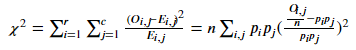
sample_dict = {'Type': ['J','J','J',
                        'B','B','B',
                        'C','C','C','C','C'], 
               'Output': [0, 1, 0, 
                          2, 0, 1,  
                          0, 0, 1, 2, 2,]}
sample_raw = pd.DataFrame(sample_dict)
sample_raw #Raw data, Output is our target variable, and Type is the category variable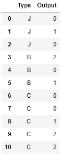

# Next, Boolean variables are generated by using unique heat coding, and the chi2 value of each boolean variable is calculated by using sklearn
sample = pd.get_dummies(sample_raw)
from sklearn.feature_selection import chi2
chi2(sample.values[:,[1,2,3]],sample.values[:,[0]])
# The first line is the chi2 value of each boolean variable

(array([0.17777778, 0.42666667, 1.15555556]),
 array([0.91494723, 0.8078868 , 0.56114397]))

# Next, the statistical chi square statistics of the original variables Type and output are calculated directly
# First, count the number of observations under each category to create a contingency table
obs_df = sample_raw.groupby(['Type','Output']).size().reset_index()
obs_df.columns = ['Type','Output','Count']
obs_df

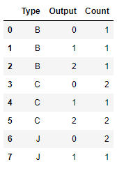
That is, the contingency table is:

from scipy.stats import chi2_contingency
obs = np.array([[1, 1, 1], [2, 1, 2],[2, 1, 0]])
chi2_contingency(obs) # The first value is the chi square statistics in the statistical significance of the variables Type and output

(1.7600000000000002,
 0.779791873961373,
 4,
 array([[1.36363636, 0.81818182, 0.81818182],
        [2.27272727, 1.36363636, 1.36363636],
        [1.36363636, 0.81818182, 0.81818182]]))

# The sum of the Boolean values calculated by the chi2 equation is the chi square statistics in the statistical sense of the original variables
chi2(sample.values[:,[1,2,3]],sample.values[:,[0]])[0].sum() == chi2_contingency(obs)[0]

True

# So how is chi2 calculated in sklearn?
# Take the first generated Boolean as an example, that is, the Type is B
# The value of chi2 is 0.1778
# This is consistent with the calculation calculated by using scipy's following code
from scipy.stats import chisquare
f_exp = np.array([5/11, 3/11, 3/11]) * 3 # A priori probability that the expected frequency is output * number of samples with Type B
chisquare([1,1,1], f_exp=f_exp) # [1,1,1] is the actual frequency of samples with Type B
# That is, chi2 in sklearn only considers the concatenated table when the Type is B

Power_divergenceResult(statistic=0.17777777777777778, pvalue=0.9149472287300311)

How to use sklearn for feature selection

import numpy as np
from sklearn.feature_selection import chi2
from sklearn.feature_selection import SelectKBest


# Load dataset directly
from sklearn.datasets import load_iris # Using iris data as demonstration data set
iris = load_iris()
X, y = iris.data, iris.target
# In this dataset, X is a continuous variable and y is a category variable
# The service conditions of chi2 are not met


# Change continuous variables to Boolean variables to meet chi2 usage conditions
# You might as well use whether it is greater than the mean to generate boolean values (for demonstration only)
X = X > X.mean(0)


# iris datasets need to be out of order before use
np.random.seed(1234)
idx = np.random.permutation(len(X))
X = X[idx]
y = y[idx]


# Select the first 100 observation points as the training set
# The rest are used as test sets
train_set = X[0:100,:]
test_set = X[100:,]
train_y = y[0:100]


# The equation is directly provided in sklearn to calculate chi square statistics
# SelectKBest will automatically select the variables with high scores based on a discriminant equation
# The discriminant equation here is F statistic
selector = SelectKBest(chi2, k=2) # K = > number of variables we want to select
selector.fit(train_set, train_y) # Train on the training set
transformed_train = selector.transform(train_set) # Transform training set
transformed_train.shape #(100, 2), which selects the third and fourth variables 
assert np.array_equal(transformed_train, train_set[:,[2,3]])


transformed_test = selector.transform(test_set) # Transform test set
assert np.array_equal(transformed_test, test_set[:,[2,3]]);
# It can be seen that the third and fourth variables are still selected for the test set

# Verify the above results
for idx in range(train_set.shape[1]):
    score, p_value = chi2(train_set[:,idx].reshape(-1,1), train_y)
    print(f"The first{idx + 1}The chi square statistics of variables and dependent variables are{round(score[0],2)}，p Value is{round(p_value[0],3)}")
# Therefore, the third and fourth variables should be selected

The chi square statistic of the first variable and dependent variable is 29.69，p The value is 0.0
 The chi square statistic of the second variable and dependent variable is 19.42，p The value is 0.0
 The chi square statistic of the third variable and dependent variable is 31.97，p The value is 0.0
 The chi square statistic of the fourth variable and dependent variable is 31.71，p The value is 0.0

1.1.1.7 F-score (classification problem)

In the classification machine learning problem, if the variable feature is a category feature, we can use the unique heat coding combined with the above chi2 method to select the most important feature. However, if the characteristic is a continuous variable, we can use ANOVA-F value. The null hypothesis of ANOVA F statistics is that if grouped by target variables (categories), the overall mean of continuous variables is the same. Therefore, we should choose continuous variables with high ANOVA-F statistics, because these continuous variables have strong correlation with the target variables.

Formula:

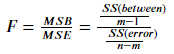
Where SS(between) is the sum of squares between groups, that is, the sum of squares between group mean and overall mean. SS(error) is the sum of squares within the group, that is, the sum of squares between the data and the group mean. m is the total number of categories of target variables and n is the number of observations.

import numpy as np
from sklearn.feature_selection import f_classif
from sklearn.feature_selection import SelectKBest


# Load dataset directly
from sklearn.datasets import load_iris # Using iris data as demonstration data set
iris = load_iris()
X, y = iris.data, iris.target
# In this dataset, X is a continuous variable and y is a category variable
# Meet the service conditions of ANOVA-F


# iris datasets need to be out of order before use
np.random.seed(1234)
idx = np.random.permutation(len(X))
X = X[idx]
y = y[idx]


# Select the first 100 observation points as the training set
# The rest are used as test sets
train_set = X[0:100,:]
test_set = X[100:,]
train_y = y[0:100]


# The equation is directly provided in sklearn to calculate ANOVA-F
# SelectKBest will automatically select the variables with high scores based on a discriminant equation
# The discriminant equation here is F statistic
selector = SelectKBest(f_classif, k=2) # K = > number of variables we want to select
selector.fit(train_set, train_y) # Train on the training set
transformed_train = selector.transform(train_set) # Transform training set
transformed_train.shape #(100, 2), which selects the third and fourth variables 
assert np.array_equal(transformed_train, train_set[:,[2,3]])


transformed_test = selector.transform(test_set) # Transform test set
assert np.array_equal(transformed_test, test_set[:,[2,3]]);
# It can be seen that the third and fourth variables are still selected for the test set

# Verify the above results
for idx in range(train_set.shape[1]):
    score, p_value = f_classif(train_set[:,idx].reshape(-1,1), train_y)
    print(f"The first{idx + 1}Of variables and dependent variables ANOVA-F The statistics are{round(score[0],2)}，p Value is{round(p_value[0],3)}")
# Therefore, the third and fourth variables should be selected

Relationship between the first variable and the dependent variable ANOVA-F The statistic is 91.39，p The value is 0.0
 Relationship between the second variable and the dependent variable ANOVA-F The statistic is 33.18，p The value is 0.0
 The third variable is related to the dependent variable ANOVA-F The statistic is 733.94，p The value is 0.0
 The fourth variable is related to the dependent variable ANOVA-F The statistic is 608.95，p The value is 0.0

1.1.1.7 Mutual Information (classification problem)

[as in 1.1.1.5] Mutual Information measures the interdependence between variables. Its essence is entropy difference, i.e???? (????) −???? (????|????)， That is, the reduction of confusion after knowing the information of another variable. Mi is equal to zero if and only if two random variables are independent. The higher the MI value, the stronger the correlation between the two variables. Compared with Pearson correlation and F statistics, it also captures nonlinear relationships.

Formula:

• If both variables are discrete:

p(????,????) (????,????) Is the joint probability mass function (PMF) of x and y, P???? (????) Is the joint probability mass function (PMF) of x.

• If both variables are continuous:

p(????,????) (????,????) Is the joint probability density function (PDF) of x and y, P???? (????) Is the joint probability density function (PDF) of x. In the case of continuous variables, in practice, the data is often discretized into buckets, and then calculated bucket by bucket.

But in fact, it is very likely that one of x and y may be a discrete variable and the other a continuous variable. Therefore, in sklearn, it is based on the nonparametric entropy estimation method based on k-nearest neighbor algorithm proposed in [1] and [2].

[1] A. Kraskov, H. Stogbauer and P. Grassberger, "Estimating mutual information". Phys. Rev. E 69, 2004.

[2] B. C. Ross "Mutual Information between Discrete and Continuous Data Sets". PLoS ONE 9(2), 2014.

import numpy as np
from sklearn.feature_selection import mutual_info_classif
from sklearn.feature_selection import SelectKBest


# Load dataset directly
from sklearn.datasets import load_iris # Using iris data as demonstration data set
iris = load_iris()
X, y = iris.data, iris.target
# In this dataset, X is a continuous variable and y is a category variable
# Meet the service conditions of MI


# iris datasets need to be out of order before use
np.random.seed(1234)
idx = np.random.permutation(len(X))
X = X[idx]
y = y[idx]


# Select the first 100 observation points as the training set
# The rest are used as test sets
train_set = X[0:100,:]
test_set = X[100:,]
train_y = y[0:100]


# The proximity number in KNN is a very important parameter
# Therefore, we rewrite a new MI calculation equation to better control this parameter
def udf_MI(X, y):
    result = mutual_info_classif(X, y, n_neighbors = 5) # The user can enter the desired number of neighbors
    return result


# SelectKBest will automatically select the variables with high scores based on a discriminant equation
# The discriminant equation here is F statistic
selector = SelectKBest(udf_MI, k=2) # K = > number of variables we want to select
selector.fit(train_set, train_y) # Train on the training set
transformed_train = selector.transform(train_set) # Transform training set
transformed_train.shape #(100, 2), which selects the third and fourth variables 
assert np.array_equal(transformed_train, train_set[:,[2,3]])


transformed_test = selector.transform(test_set) # Transform test set
assert np.array_equal(transformed_test, test_set[:,[2,3]]);
# It can be seen that the third and fourth variables are still selected for the test set

# Check the above results
for idx in range(train_set.shape[1]):
    score = mutual_info_classif(train_set[:,idx].reshape(-1,1), train_y, n_neighbors = 5)
    print(f"The first{idx + 1}The mutual information between variables and dependent variables is{round(score[0],2)}")
# Therefore, the third and fourth variables should be selected

The mutual information between the first variable and the dependent variable is 0.56
 The mutual information between the second variable and the dependent variable is 0.28
 The mutual information between the third variable and the dependent variable is 0.99
 The mutual information between the fourth variable and the dependent variable is 1.02

Column series:

Column | Jupyter Based Feature Engineering Manual: data preprocessing (I)

Column | Jupyter Based Feature Engineering Manual:Data preprocessing (II)

Column | Jupyter Based Feature Engineering Manual: data preprocessing (III)

Column | Jupyter Based Feature Engineering Manual: data preprocessing (IV)

Column | Jupyter Based Feature Engineering Manual: feature selection (I)

At present, the complete Chinese version of the project is being produced. Please keep an eye on it~

Chinese Jupyter address:

https://github.com/YC-Coder-Chen/feature-engineering-handbook/blob/master/ Chinese Version / 2.% 20 feature selection ipynb