Introduction: This paper discusses how to combine the contour area method with the edge brightness curve modeling method in the process of detecting the diameter of the ring in the metal template to see whether the accuracy of the ring can be improved. From the test results, it does not show the advantages of the two combination methods.
Key words: ring detection, boundary area, center
§ 01 ring detection
1.1 problem background
in Using edge gray change modeling to improve the accuracy of ring diameter This paper discusses the method to increase the measurement accuracy by modeling the brightness change of the ring boundary in the picture of bacteriostatic ring metal template. Final certificate:
- This method can improve the circle radius obtained by HoughCircles transform;
- But compared to Measuring circular radius by circular contour area For the above method, the area measurement accuracy has not been achieved by using the transformation brightness change modeling.
therefore, the next question remains: can these two methods be combined to finally improve the measurement accuracy?
1.1.1 method combination
there are two ways to combine edge brightness modeling and contour area statistics:
1. Using the parameters in the edge brightness modeling to provide the binarization threshold in the contour area;
2. The center point of contour area is used to provide the center point for edge brightness modeling;
the following is an experimental study to verify whether the combination of the above two methods is effective.
1.2 contour area method
the processing program comes from Measuring circular radius by circular contour area The final handler of the blog post. The processed picture data is 100 pieces of data obtained by the diagonal translation of the template above the scanning.
1.2.1 contour area calculation circular radius
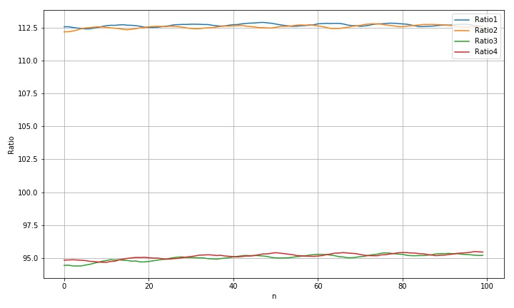
the following is the change of the circular radius calculated by the contour area with the diagonal translation of the metal template on the scanner surface. It can be seen that the radius data of both large and small circles fluctuate periodically with translation, and the fluctuation phases of the two circles are just complementary, showing a phase difference of about 180 °.
1.2.2 take the average radius of large circle and small circle
according to the above fluctuations, divide two large circles and two small circles into two groups, average them, and check the change of values after average.
the following figure shows the change of measurement curve after averaging the large circle and the small circle respectively:
- Indeed, the original volatility has been greatly reduced;
- But the fluctuation has not completely disappeared;
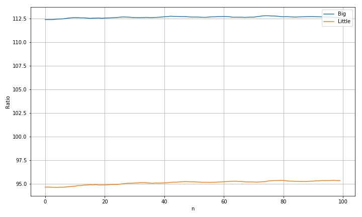
the data range after average is shown below:
max(r1a)-min(r1a): 0.409755637718888
max(r2a)-min(r2a): 0.742439612301439
the following is the variance and range corresponding to the original four circle radii. It can be seen that after the average value, these ranges are also relatively reduced.
std(rdim1): 0.10686994419992152
std(rdim2): 0.12228622717628217
std(rdim3): 0.24442592829855
std(rdim4): 0.2037604935717777
max(rdim1)-min(rdim1): 0.49655149847501434
max(rdim2)-min(rdim2): 0.6161167744770495
max(rdim3)-min(rdim3): 0.9954571335234874
max(rdim4)-min(rdim4): 0.8185206978833861
however, the reason for the small decrease is that there is still a trend of large data increase on the basis of the original data fluctuation. This change has become a major contribution to the poor data.
§ 02 method fusion
2.1 the first fusion scheme
the first fusion scheme is to use circular edge gray modeling to estimate the threshold of image segmentation through modeling parameters.
2.1.1 code change
#------------------------------------------------------------

cealldiag = '/home/aistudio/work/Scanner/cealldiag.npz'
cealldata = load(cealldiag, allow_pickle=True)
ceall = cealldata['ceall']

#------------------------------------------------------------

def sigmoidx(x, a,b,c,d):
    return a/(1+exp(-(x-c)*d)) + b

#------------------------------------------------------------
block_side = 140
def img2block(img, circles):
    block = []
    for c in circles:
        left = int(c[0] - block_side)
        right = left + block_side*2
        top = int(c[1] - block_side)
        bottom = top + block_side*2

        block.append(img[top:bottom, left:right, :])

    return block

#------------------------------------------------------------
rdim1 = []
rdim2 = []
rdim3 = []
rdim4 = []

threshold = 100
threshdim = []

for id,f in tqdm(enumerate(allfile)):
    img = cv2.imread(f)
    cc = alldim[id]
    ce = ceall[id]

#    if id >= 41: break

    #--------------------------------------------------------
'''
    for c in cc:
        printt(c:)
        cv2.circle(img, (c[0], c[1]), int(c[2]), (0,0,255), 10)

    plt.figure(figsize=(10,10))
    plt.imshow(img[:,:,::-1])

    break
'''
    #--------------------------------------------------------

    block = img2block(img, cc)

    #--------------------------------------------------------
'''
    plt.figure(figsize=(10,10))
    plt.subplot(2,2,1)
    plt.imshow(block[0])
    plt.subplot(2,2,2)
    plt.imshow(block[1])
    plt.subplot(2,2,3)
    plt.imshow(block[2])
    plt.subplot(2,2,4)
    plt.imshow(block[3])

    plt.savefig('/home/aistudio/stdout.jpg')
    break
'''
    #--------------------------------------------------------

#    plt.figure(figsize=(10,10))

    ratioDim = []
    x = linspace(0, 100, 100, endpoint=False)
    for iidd,b in enumerate(block):

        y = ce[iidd]
        param = [140, 20, 50, 0.2]
        param, conv=curve_fit(sigmoidx, x,  y, p0=param)

        bgray = cv2.cvtColor(b, cv2.COLOR_BGR2GRAY)
#        threshold = mean(bgray.flatten())
        threshold = (param[0]/2+param[1])
        threshdim.append(threshold)

        ret,thresh = cv2.threshold(bgray, threshold, 255, 0)
        contours,hierarchy = cv2.findContours(thresh, cv2.RETR_TREE, cv2.CHAIN_APPROX_NONE)
        cv2.drawContours(b, contours, -1, (0, 0, 255), 3)

        areaDim = []
        for id,c in enumerate(contours):
            areaDim.append(cv2.contourArea(c))

        asorted = sorted(areaDim)
        a = asorted[-2]
        r = sqrt(a/pi)
        ratioDim.append(r)

#        plt.subplot(2,2,iidd+1)
#        plt.hist(bgray.flatten(), bins=20)
#        plt.imshow(b[:,:,::-1])

#    printt(ratioDim:)
    if len(ratioDim) != 4:
        printt(ratioDim:)
        break

    rdim1.append(ratioDim[0])
    rdim2.append(ratioDim[1])
    rdim3.append(ratioDim[2])
    rdim4.append(ratioDim[3])

#    plt.savefig('/home/aistudio/stdout.jpg')
#    plt.show()

#    break
2.1.2 treatment results
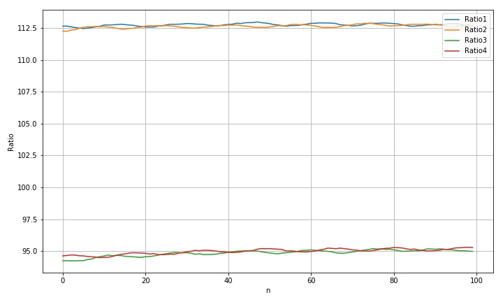
max(r1a)-min(r1a): 0.42009826663701233
max(r2a)-min(r2a): 0.7635241870300433
std(rdim1): 0.10759563831366077
std(rdim2): 0.12086249841122422
std(rdim3): 0.24667243762087157
std(rdim4): 0.21136071101720186
max(rdim1)-min(rdim1): 0.5210168958673478
max(rdim2)-min(rdim2): 0.619309102259777
max(rdim3)-min(rdim3): 0.95698803317228
max(rdim4)-min(rdim4): 0.8067502496432724
whether from the processing data curve or from the final statistics, this combination has not improved. The improvement effect is very weak.
2.2 the second scheme
the second scheme is to use the center of the boundary to correct the center point in the modeling of edge brightness curve.
2.2.1 find the boundary Center
in the blog OpenCV center of contour Using CV2 The moments function calculates the method in contoursde.
M = cv2.moments(c)
m00 = M['m00']

if m00 > 0:
    cX = M['m10'] / M['m00']
    cY = M['m01'] / M['m00']
else:
    cX = 0
    cY = 0
use the above method to obtain the center point of the circular boundary.
(1) Processing results
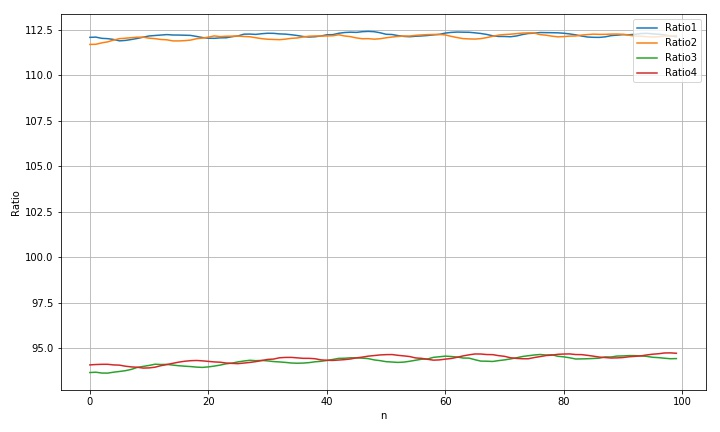
std(rdim1): 0.111475597768182
std(rdim2): 0.12480667032700701
std(rdim3): 0.2491116756143372
std(rdim4): 0.21128501595131527
max(rdim1)-min(rdim1): 0.5198071417283359
max(rdim2)-min(rdim2): 0.6324433245598016
max(rdim3)-min(rdim3): 1.0217870978580805
max(rdim4)-min(rdim4): 0.8341840265537286
according to the result analysis, this combination method has not achieved obvious results. The results are basically consistent with those obtained by using the boundary center directly.
※ general ※ conclusion ※
this paper discusses whether the accuracy of the ring can be improved by combining the contour area method with the edge brightness curve modeling method in the process of detecting the ring diameter in the metal template. From the test results, it does not show the advantages of the two combination methods.
■ links to relevant literature:
- Using edge gray change modeling to improve the accuracy of ring diameter
- Calculate the radius of the ring by using the contour area of the circle: CV2 findContours, contourArea
- OpenCV center of contour
● links to relevant charts:
- Figure 1.2.1 data of circular radius obtained by contour area
- The measurement results corresponding to the average values of two large circles and two small circles
- Figure 2.1.1 processing results
- Figure 2.2.1 processing results
processing program
#!/usr/local/bin/python
# -*- coding: gbk -*-
#============================================================
# TEST1.PY                     -- by Dr. ZhuoQing 2022-01-26
#
# Note:
#============================================================

from headm import *                 # =
import cv2
from tqdm import tqdm
from scipy.optimize     import curve_fit


#------------------------------------------------------------
npzdiag = '/home/aistudio/work/Scanner/ScanDiagBlock.npz'
scandiagdir = '/home/aistudio/work/Scanner/ScanDiagBlock'
#npzdiag = '/home/aistudio/work/Scanner/ScanRowBlock.npz'
#scandiagdir = '/home/aistudio/work/Scanner/ScanRowBlock'
#npzdiag = '/home/aistudio/work/Scanner/ScanVertBlock.npz'
#scandiagdir = '/home/aistudio/work/Scanner/ScanVertBlock'

#filedim = sorted([s for s in os.listdir(scandiagdir) if s.find("jpg") > 0])
#printt(filedim:)

alldata = load(npzdiag, allow_pickle=True)
#printt(alldata.files:)
alldim = alldata['alldim']
allfile = alldata['allfile']

#printt(alldim:, allfile:)

#------------------------------------------------------------

cealldiag = '/home/aistudio/work/Scanner/cealldiag.npz'
cealldata = load(cealldiag, allow_pickle=True)
ceall = cealldata['ceall']

#------------------------------------------------------------

def sigmoidx(x, a,b,c,d):
    return a/(1+exp(-(x-c)*d)) + b


#------------------------------------------------------------
block_side = 140
def img2block(img, circles):
    block = []
    for c in circles:
        left = int(c[0] - block_side)
        right = left + block_side*2
        top = int(c[1] - block_side)
        bottom = top + block_side*2

        block.append(img[top:bottom, left:right, :])

    return block

#------------------------------------------------------------
CIRCLE_NUM          = 100
DELTA_RATIO         = 7
SAMPLE_NUM          = 300
theta = linspace(0, 2*pi, SAMPLE_NUM)
def circleEdges(img, circles, xy):
    clight = []
    for iidd,c in enumerate(circles):
        rdim = linspace(c[-1]-DELTA_RATIO, c[-1]+DELTA_RATIO, CIRCLE_NUM)
        rmean = []
        xx = xy[iidd][0]
        yy = xy[iidd][1]

        for id,r in enumerate(rdim):
            thetadim = []
            for a in theta:
                x = int(xx + r*cos(a))
                y = int(yy + r*sin(a))
                thetadim.append(img[y,x])
            rmean.append(mean(thetadim))
        clight.append(rmean)
    return clight


#------------------------------------------------------------
rdim1 = []
rdim2 = []
rdim3 = []
rdim4 = []

threshold = 100
for id,f in tqdm(enumerate(allfile)):
    img = cv2.imread(f)
    gray = cv2.cvtColor(img, cv2.COLOR_BGR2GRAY)


    cc = alldim[id]
    rdim = alldim[id]
    ce = ceall[id]

    block = img2block(img, cc)
    x = linspace(0, 100, 100, endpoint=False)
    xydim = []

    for iidd,b in enumerate(block):
        bgray = cv2.cvtColor(b, cv2.COLOR_BGR2GRAY)
        threshold = mean(bgray.flatten())

        ret,thresh = cv2.threshold(bgray, threshold, 255, 0)
        contours,hierarchy = cv2.findContours(thresh, cv2.RETR_TREE, cv2.CHAIN_APPROX_NONE)
        cv2.drawContours(b, contours, -1, (0, 0, 255), 3)

        areaDim = []
        momentDim = []

        bcc = cc[iidd]
        bx = bcc[0] - block_side
        by = bcc[1] - block_side

        for id,c in enumerate(contours):
            areaDim.append(cv2.contourArea(c))

            M = cv2.moments(c)
            m00 = M['m00']

            if m00 > 0:
                cX = M['m10'] / M['m00']
                cY = M['m01'] / M['m00']
            else:
                cX = 0
                cY = 0


            momentDim.append((cX + bx,cY + by))

        asorted = sorted(list(zip(areaDim, momentDim)), key=lambda x:x[0])
#        printt(len(asorted))
        a = asorted[-2][0]
        xydim.append(asorted[-2][1])

    #--------------------------------------------------------
#    img = cv2.imread(f)
#    gray = cv2.cvtColor(img, cv2.COLOR_BGR2COLOR)

    ce = circleEdges(gray, cc, xydim )
    x = linspace(0, 100, 100, endpoint=False)
    N = 100
    delta=7
    ratioDim = []
    for i,c in enumerate(ce):
        y = c
#        printt(c:)
        param = (140, 20, 50, 0.2)
        param, conv = curve_fit(sigmoidx, x, y, p0=param)
        r0 = rdim[i][-1]
        rmod = r0 + (param[2] - N/2)*(2*delta/N)
        ratioDim.append(rmod)

    #--------------------------------------------------------
    rdim1.append(ratioDim[0])
    rdim2.append(ratioDim[1])
    rdim3.append(ratioDim[2])
    rdim4.append(ratioDim[3])


#    break


#------------------------------------------------------------
r1a = (array(rdim1) + array(rdim2)) / 2
r2a = (array(rdim3) + array(rdim4)) / 2

printt(max(r1a)-min(r1a):)
printt(max(r2a)-min(r2a):)

#------------------------------------------------------------
plt.clf()
plt.figure(figsize=(10,6))
plt.plot(rdim1, label='Ratio1')
plt.plot(rdim2, label='Ratio2')
plt.plot(rdim3, label='Ratio3')
plt.plot(rdim4, label='Ratio4')
#plt.plot(r1a, label='Big')
#plt.plot(r2a, label='Little')
plt.legend(loc="upper right")
plt.xlabel("n")
plt.ylabel("Ratio")
plt.grid(True)
plt.tight_layout()
plt.savefig('/home/aistudio/stdout.jpg')
plt.show()


#------------------------------------------------------------
printt(std(rdim1):,std(rdim2):,std(rdim3):,std(rdim4):)
printt(max(rdim1)-min(rdim1):)
printt(max(rdim2)-min(rdim2):)
printt(max(rdim3)-min(rdim3):)
printt(max(rdim4)-min(rdim4):)


#------------------------------------------------------------
#        END OF FILE : TEST1.PY
#============================================================