Activation function:
The principle of activation layer is to add nonlinear activation function after the output of other layers to increase the nonlinear ability of the network and improve the ability of neural network to fit complex functions. The selection of activation function is very important for the training of neural network. The commonly used activation functions include Sigmoid function, Tanh function, ReLU function and LeakyReLU. The activation layer simulates the stimulation process of biological nervous system, and introduces the nonlinear function, so as to characterize the characteristics more effectively. In the convolution layer and full connection layer of convolution neural network, the output value of each layer is essentially the result of calculating the weighted average value of the input neuron. Because the weighted average is a linear operation, after the combination and superposition of multiple convolution layers or full connection layers, the obtained function is still a linear transformation function. Therefore, in order to further enhance the expression ability of convolutional neural network, it is necessary to add the activation function with nonlinear characteristics to the structure of convolutional neural network. Some common activation functions are described below
Learning content:
Sigmoid
Sigmoid function is a common S-type function in biology, and the function curve is shown in the figure below. It can transform the input number to 0 ~ 1 for output. If the input is a particularly small negative number, the output is 0. If the input is a particularly large positive number, the output is 1. Sigmoid can be regarded as a nonlinear activation function to endow the network with nonlinear discrimination ability, which is often used in binary classification.

The calculation formula of Sigmoid activation function can be expressed as formula (2-1), where x represents the input pixel. By analyzing the function expression and Sigmoid curve, we can know that the advantage of Sigmoid activation function is that the curve is smooth and derivative everywhere; The disadvantage is that the operation of power function is slow and the calculation of activation function is large; When calculating the reverse gradient, the gradient of Sigmoid is very gentle in the saturated region, which is easy to create the problem of gradient disappearance and slow down the convergence speed.

import matplotlib.pyplot as plt
import numpy as np

def Sigmoid(x):
    y = np.exp(x) / (np.exp(x) + 1)
    return y

if __name__ == '__main__':

    x = np.arange(-10, 10, 0.01)

    plt.plot(x, Sigmoid(x), color = '#00ff00')
    plt.title("Sigmoid")
    plt.grid()
    plt.savefig("Sigmoid.png", bbox_inches='tight')
    plt.show()
Tanh
If the input and output of a function with - 1 as shown in the figure below is an odd number, and the input and output of a function with - 1 as a continuous number, especially if it is a function with - 1 as an odd number; The problem that the mean value of Sigmoid function is not 0 is solved. Tanh can be used as a nonlinear activation function to give the network nonlinear discrimination ability.
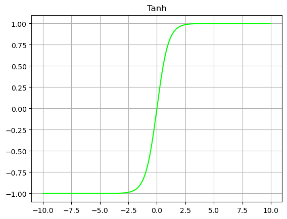
The calculation formula of Tanh activation function can be expressed by formula (2-2), where x represents input. By analyzing the function expression and Tanh curve, we can know that the advantage of Tanh activation function is that the curve is smooth, derivative everywhere, has good symmetry, and the network mean value is 0. The Tanh function is similar to the Sigmoid function in that the power function is operated slowly and the calculation of the activation function is large; When calculating the reverse gradient, the gradient of Tanh is very gentle in the saturated region, which is easy to create the problem of gradient disappearance and slow down the convergence speed.

import matplotlib.pyplot as plt
import numpy as np

def Tanh(x):
    y = (np.exp(x) - np.exp(-x)) / (np.exp(x) + np.exp(-x))
    # y = np.tanh(x)
    return y

if __name__ == '__main__':

    x = np.arange(-10, 10, 0.01)

    plt.plot(x, Tanh(x), color = '#00ff00')
    plt.title("Tanh")
    plt.grid()
    plt.savefig("Tanh.png", bbox_inches='tight')
    plt.show()
ReLU
The rectified linear unit (ReLU) is an activation function commonly used in deep neural networks. The curve of ReLU function is shown in the figure below. The whole function can be divided into two parts. In the part less than 0, the output of the activation function is 0; In the part greater than 0, the output of the activation function is the input.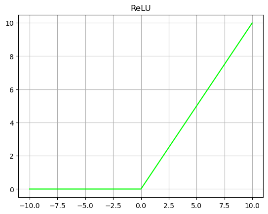
The calculation formula of ReLU activation function can be expressed by formula (2-3), where x represents input. By analyzing the function expression and ReLU curve, we can know that the advantages of ReLU activation function are fast convergence speed, no saturation interval, and the gradient is fixed to 1 in the part greater than 0, which effectively solves the problem of gradient disappearance in Sigmoid. The calculation speed is fast. ReLU only needs a threshold to get the activation value without calculating a lot of complex exponential operations. It has biological like properties. The disadvantage of ReLU function is that it may "die" during training. If a very large gradient passes through a ReLU neuron, after updating the parameters, the value of this neuron is less than 0. At this time, ReLU will no longer activate any data. If this happens, then all gradients flowing through the neuron will become 0. Setting the learning rate reasonably will reduce the probability of this situation.

import matplotlib.pyplot as plt
import numpy as np

def ReLU(x):
    y = np.where(x < 0, 0, x)
    return y

if __name__ == '__main__':

    x = np.arange(-10, 10, 0.01)

    plt.plot(x, ReLU(x), color = '#00ff00')
    plt.title("ReLU")
    plt.grid()
    plt.savefig("ReLU.png", bbox_inches='tight')
    plt.show()
LeakyReLU
Leaky ReLU is an improved version of the ReLU function. Ordinary ReLU sets all negative values to zero, while leaky ReLU gives all negative values a non-zero slope. In the process of back propagation, the gradient can also be calculated for the part where the input of leaky ReLU activation function is less than zero The problem of gradient disappearance is avoided. The image of LeakyReLU activation function is shown in Figure 2-8.
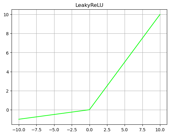
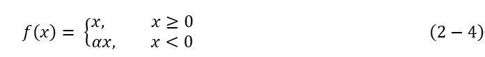
The calculation formula of LeakyReLU activation function can be expressed as (2-4), where x represents input. Through the function expression and LeakyReLU curve, we can know that LeakyReLU has the advantages of ReLU; The problem of ReLU function is solved to prevent the emergence of dead neurons. The disadvantage is α Parameters need to be selected manually, and specific values need to be selected according to the needs of the task.
import matplotlib.pyplot as plt
import numpy as np

def LeakyReLU(x, a):
    # The a parameter of LeakyReLU cannot be trained and is specified artificially.
    y = np.where(x < 0, a * x, x)
    return y

if __name__ == '__main__':

    x = np.arange(-10, 10, 0.01)

    plt.plot(x, LeakyReLU(x, 0.1), color = '#00ff00')
    plt.title("LeakyReLU")
    plt.grid()
    plt.savefig("LeakyReLU.png", bbox_inches='tight')
    plt.show()
ELU
The curve of ELU activation function is shown in the figure below. The gradient of the part with input greater than 0 is 1, and the part with input less than 0 is infinitely close to - a. The ideal activation function should satisfy that the distribution of output is zero mean, which can speed up the training speed. The activation function is one-sided saturated and can converge better. The ELU activation function meets these two characteristics at the same time. In the fourth chapter of this paper, we will use the ELU activation function in the design of encoder decoder network.
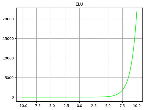
The calculation formula of ELU activation function can be expressed as formula (2-5), where x is the input. By analyzing the function expression and the ELU function curve, we can know that the output of the function is distributed with zero mean value, so it can be used alone. There is no need to add BN layer in front. The ELU function has single saturation and can converge better. Since ELU involves exponential operation, the reasoning speed is relatively time-consuming.
import matplotlib.pyplot as plt
import numpy as np

def ELU(x, a):
    y = np.where(x < 0, x, a*(np.exp(x)-1))
    return y

if __name__ == '__main__':

    x = np.arange(-10, 10, 0.01)

    plt.plot(x, ELU(x, 1),  color = '#00ff00')
    plt.title("ELU")
    plt.grid()
    plt.savefig("ELU.png", bbox_inches='tight')
    plt.show()
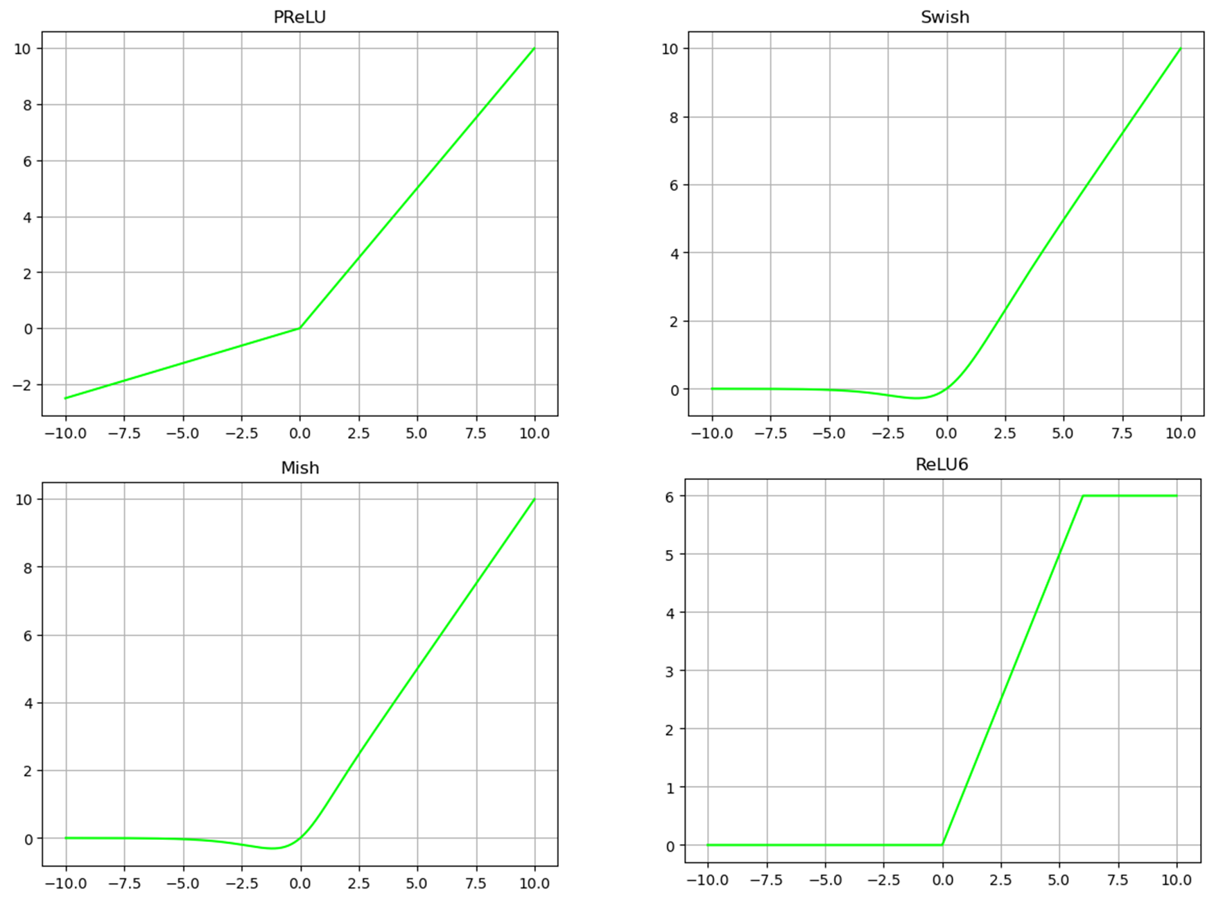
Other activation functions
PReLU,ReLU6,Swish,Mish
Other activation functions are proposed under the improvement of the above activation functions. I put the code below
import matplotlib.pyplot as plt
import numpy as np


def Sigmoid(x):
    y = np.exp(x) / (np.exp(x) + 1)
    return y


def Tanh(x):
    y = (np.exp(x) - np.exp(-x)) / (np.exp(x) + np.exp(-x))
    # y = np.tanh(x)
    return y


def ReLU(x):
    y = np.where(x < 0, 0, x)
    return y


def LeakyReLU(x, a):
    # The a parameter of LeakyReLU cannot be trained and is specified artificially.
    y = np.where(x < 0, a * x, x)
    return y

def ELU(x, a):
    y = np.where(x < 0, x, a*(np.exp(x)-1))
    return y


def PReLU(x, a):
    # The a parameter of PReLU can be trained
    y = np.where(x < 0, a * x, x)
    return y


def ReLU6(x):
    y = np.minimum(np.maximum(x, 0), 6)
    return y


def Swish(x, b):
    y = x * (np.exp(b * x) / (np.exp(b * x) + 1))
    return y


def Mish(x):
    # Mish here has been reduced by e and ln
    temp = 1 + np.exp(x)
    y = x * ((temp * temp - 1) / (temp * temp + 1))
    return y


def Grad_Swish(x, b):
    y_grad = np.exp(b * x) / (1 + np.exp(b * x)) + x * (b * np.exp(b * x) / ((1 + np.exp(b * x)) * (1 + np.exp(b * x))))
    return y_grad


def Grad_Mish(x):
    temp = 1 + np.exp(x)
    y_grad = (temp * temp - 1) / (temp * temp + 1) + x * (4 * temp * (temp - 1)) / (
                (temp * temp + 1) * (temp * temp + 1))
    return y_grad


if __name__ == '__main__':
    x = np.arange(-10, 10, 0.01)

    plt.plot(x, Sigmoid(x), color = '#00ff00')
    plt.title("Sigmoid")
    plt.grid()
    plt.savefig("Sigmoid.png", bbox_inches='tight')
    plt.show()

    plt.plot(x, Tanh(x), color = '#00ff00')
    plt.title("Tanh")
    plt.grid()
    plt.savefig("Tanh.png", bbox_inches='tight')
    plt.show()

    plt.plot(x, ReLU(x), color = '#00ff00')
    plt.title("ReLU")
    plt.grid()
    plt.savefig("ReLU.png", bbox_inches='tight')
    plt.show()

    plt.plot(x, LeakyReLU(x, 0.1), color = '#00ff00')
    plt.title("LeakyReLU")
    plt.grid()
    plt.savefig("LeakyReLU.png", bbox_inches='tight')
    plt.show()

    plt.plot(x, ELU(x, 1),  color = '#00ff00')
    plt.title("ELU")
    plt.grid()
    plt.savefig("ELU.png", bbox_inches='tight')
    plt.show()

    plt.plot(x, PReLU(x, 0.25), color = '#00ff00')
    plt.title("PReLU")
    plt.grid()
    plt.savefig("PReLU.png", bbox_inches='tight')
    plt.show()

    plt.plot(x, ReLU6(x), color = '#00ff00')
    plt.title("ReLU6")
    plt.grid()
    plt.savefig("ReLU6.png", bbox_inches='tight')
    plt.show()

    plt.plot(x, Swish(x, 1), color = '#00ff00')
    plt.title("Swish")
    plt.grid()
    plt.savefig("Swish.png", bbox_inches='tight')
    plt.show()

    plt.plot(x, Mish(x), color = '#00ff00')
    plt.title("Mish")
    plt.grid()
    plt.savefig("Mish.png", bbox_inches='tight')
    plt.show()


    plt.plot(x, Grad_Mish(x))
    plt.plot(x, Grad_Swish(x, 1))
    plt.title("Gradient of Mish and Swish")
    plt.legend(['Mish', 'Swish'])
    plt.grid()
    plt.savefig("MSwith.png", bbox_inches='tight')
    plt.show()