Shur complement is undoubtedly a simple and easy-to-use method, but the projection theorem has routines, which is more cool.
Nonsingular description is better, but singularity can reduce the coupling term.
Now I only master the general system simulation of Shur complement. Singularity and projection are not good.
To sum up, there are three types:
1. Shur supplement general system (common, available);
2. Shur complement singular system (I'm not sure whether this kind is feasible, I think it is feasible, but I haven't seen it);
3. Projection theorem singular system (used by Mr. Wang, with Mr. Wang program).
Mr. Wang, the simplest program, put it first
clear all;           % This The convex optimization algorithm is solved by invoking the solver MOSEK through YALMIP.
yalmip('clear');
[A,B,E,C,D,F,rule,b_min,b_max,v_max]=exp_sys; % system matrices of Type-2 Fuzzy systems

mu_1=[1;1;1;1];   % stablity

[~,n_d]=size(B{1});
[~,n_f]=size(E{1});
n_r=1;
[n_y,n_x]=size(C{1});

H1=[mu_1(1)*eye(n_x);mu_1(2)*eye(n_x);mu_1(3)*eye(n_x);mu_1(4)*eye(n_x)];

P=sdpvar(2*n_x,2*n_x);

G1=sdpvar(n_x,n_x,'full');

for s=1:1:rule
    X{s}=sdpvar(4*n_x,n_x,'full');
    barAF{s}=sdpvar(n_x,n_x,'full');
    barBF{s}=sdpvar(n_x,n_y,'full');
end

for s=1:1:rule
    for k=1:1:rule
        Xi_1{s}{k}=[zeros(2*n_x,2*n_x) P;P zeros(2*n_x,2*n_x)]...
        +[-X{k} -H1*G1 X{k}*A{s}+H1*barBF{k}*C{k} H1*barAF{k}]...
        +[-X{k} -H1*G1 X{k}*A{s}+H1*barBF{k}*C{k} H1*barAF{k}]';
    end
end

LMI_S= [lmi(P>=0):'P'];

for s=1:1:rule
    for k=1:1:rule
     LMI_S=LMI_S+[lmi(Xi_1{s}{k}<=0):'LMI_S'];
    end
end

options = sdpsettings('solver','mosek','shift','0.00');
solution = optimize(LMI_S, [],options)
check(LMI_S)
There are also some problems with this program, mainly The performance index is too small, and the calculated margin is positive
It should be the right procedure. This is my target program.
Procedure of Shur complement theorem (only considered)Output feedback of)
clear all;yalmip('clear');

A=[0.1 0.4;0.8 0.9];B=[1;1];C=[1 0];D1=[1;0];CZ=[1 0];D2=[0];

n_x=2;
n_d=1;
theta=6.0490e-2;
gamma_2=sdpvar(1,1,'full');
P=sdpvar(n_x,n_x);
Y=sdpvar(n_d,n_d);
G=sdpvar(n_d,n_x);

Q=[-P              zeros(n_x,n_d)    (P*A+B*G)'   CZ' ;
    zeros(n_d,n_x) -gamma_2*eye(n_d) (P*D1)'      D2' ;
    (P*A+B*G)      (P*D1)            -P          zeros(n_x,n_d);
    CZ             D2                zeros(n_d,n_x) -eye(n_d) ];

Theta=[-theta*eye(n_d) (P*B-B*Y)';
    (P*B-B*Y) -eye(n_x)];

LMI_S= [lmi(gamma_2>=0):'gamma_2'];
LMI_S= LMI_S+[lmi(P>=0):'P'];
LMI_S= LMI_S+[lmi(Q<=0):'Q'];
LMI_S= LMI_S+[lmi(Theta<=0):'Theta'];


options = sdpsettings('solver','mosek','shift','0.00');
solution = optimize(LMI_S, gamma_2,options)
check(LMI_S)

gamma_2= sqrt(value(gamma_2))
Everything is normal after this calculation.
I'm going to write this in a projection singular system.
Projection singular system program
% This The convex optimization algorithm is solved by invoking the solver MOSEK through YALMIP.
clear all;yalmip('clear');

A=[0.1 0.4;-0.8 0.9];B=[1;1];C1=[1 0];D1=[0.1;0];C2=[0.1 0.2];D2=[0];

[~,n_u]=size(B);
[n_y,n_x]=size(C1);
n_d=1;n_z=1;

mu_1=[1;1];
H0=[eye(n_x) zeros(n_x,n_u);zeros(n_u,n_x) zeros(n_u,n_u)];
H1=[zeros(n_x,n_u);mu_1(1)*eye(n_u);zeros(n_d,n_u);zeros(n_x,n_u);mu_1(2)*eye(n_u);zeros(n_d,n_u)];

gamma2=sdpvar(1,1,'full');
P=sdpvar(n_x+n_u,n_x+n_u);
X11=sdpvar(2*(n_x+n_u+n_d),n_x,'full');
G=sdpvar(n_u,n_u,'full');
X2=sdpvar(2*(n_x+n_u+n_d),n_z,'full');
GK=sdpvar(n_u,n_y,'full');

Psi_d=[P                     zeros(n_x+n_u,n_d);
       zeros(n_d,n_x+n_u)    eye(n_d,n_d)];
Sigma_d=mdiag(Psi_d,-H0'*P*H0,-gamma2*eye(n_d));

Xi=Sigma_d...
    +[-X11 -H1*G -X2 [X11*A+H1*GK*C1+X2*C2 X11*B-H1*G] X11*D1+X2*D2]...
    +[-X11 -H1*G -X2 [X11*A+H1*GK*C1+X2*C2 X11*B-H1*G] X11*D1+X2*D2]';

LMI_S= [lmi(gamma2>=0):'gamma_d'];
LMI_S= LMI_S+[lmi(P>=0):'P'];
LMI_S=LMI_S+[lmi(Xi<=0):'LMI_S'];

options = sdpsettings('solver','mosek','shift','0.00');
solution = optimize(LMI_S, [],options)
check(LMI_S)

gamma=value(gamma2)

GG=value(G)
GGKK=value(GK)
K=inv(GG)*GGKK
A
eig(A)
AA=A+B*K*C1
eig(AA)

figure()
x=[1;1];
for i=1:1:20
    X(:,i)=x;
    x=AA*x;
end
plot(X(1,:))
solution =
With the following fields struct:
yalmiptime: 0.5856
solvertime: 0.5524
info: 'Successfully solved (MOSEK)'
problem: 0
++++++++++++++++++++++++++++++++++++++++++++++++++++++++++++++++++++++++++++++++
| ID| Constraint| Primal residual| Dual residual| Tag|
++++++++++++++++++++++++++++++++++++++++++++++++++++++++++++++++++++++++++++++++
| #1| Elementwise inequality| 1.2536| -2.0462e-10| gamma_d|
| #2| Matrix inequality| 4.8449e-11| 1.7906e-10| P|
| #3| Matrix inequality| -1.832e-10| 6.0818e-10| LMI_S|
++++++++++++++++++++++++++++++++++++++++++++++++++++++++++++++++++++++++++++++++
gamma =
1.2536
GG =
1.0445
GGKK =
-0.1090
K =
-0.1043
A =
0.1000 0.4000
-0.8000 0.9000
ans =
0.5000 + 0.4000i
0.5000 - 0.4000i
AA =
-0.0043 0.4000
-0.9043 0.9000
ans =
0.4478 + 0.3966i
0.4478 - 0.3966i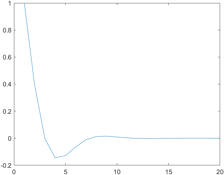
Output feedback, considerPerformance.
Solvable, the margin is also right,The performance is 1.1196, and the eigenvalue is also stable and OK - but it seems different from the previous Shur supplement. Moreover, it won't work again after changing the system.
Therefore, it is necessary for me to compare the procedures supplemented by Shur. If it's done, it's done. If it's not done, it's done.
Shur complement nonsingular system program
clear all;yalmip('clear');

A=[0.1 0.4;-0.8 0.9];B=[1;1];C1=[1 0];D1=[0.1;0];C2=[0.1 0.2];D2=[0];

[n_y,n_x]=size(C1);
n_d=1;
theta=6.0490e-12;
gamma_2=sdpvar(1,1,'full');
P=sdpvar(n_x,n_x);
Y=sdpvar(n_d,n_d);
G=sdpvar(n_d,n_y);

Q=[-P              zeros(n_x,n_d)    (P*A+B*G*C1)'  C2'           ;
    zeros(n_d,n_x) -gamma_2*eye(n_d) (P*D1)'        D2'           ;
    (P*A+B*G*C1)   (P*D1)            -P             zeros(n_x,n_d);
    C2             D2                zeros(n_d,n_x) -eye(n_d)    ];

Theta=[-theta*eye(n_d) (P*B-B*Y)';
    (P*B-B*Y) -eye(n_x)];

LMI_S= [lmi(gamma_2>=0):'gamma_2'];
LMI_S= LMI_S+[lmi(P>=0):'P'];
LMI_S= LMI_S+[lmi(Q<=0):'Q'];
LMI_S= LMI_S+[lmi(Theta<=0):'Theta'];


options = sdpsettings('solver','mosek','shift','0.00');
solution = optimize(LMI_S, gamma_2,options)
check(LMI_S)

gamma_2= sqrt(value(gamma_2))

GG=value(G)
YY=value(Y)
K=inv(YY)*GG
A
eig(A)
AA=A+B*K*C1
eig(AA)

x=[1;1];
for i=1:1:20
    X(:,i)=x;
    x=AA*x;
end
plot(X(1,:))
solution =
With the following fields struct:
yalmiptime: 0.5993
solvertime: 0.5677
info: 'Successfully solved (MOSEK)'
problem: 0
++++++++++++++++++++++++++++++++++++++++++++++++++++++++++++++++++++++++++++++++
| ID| Constraint| Primal residual| Dual residual| Tag|
++++++++++++++++++++++++++++++++++++++++++++++++++++++++++++++++++++++++++++++++
| #1| Elementwise inequality| 0.0023246| 1.4488e-05| gamma_2|
| #2| Matrix inequality| 0.078725| 9.1758e-08| P|
| #3| Matrix inequality| 2.8546e-08| 3.8475e-08| Q|
| #4| Matrix inequality| -7.1817e-09| 3.0763e-08| Theta|
++++++++++++++++++++++++++++++++++++++++++++++++++++++++++++++++++++++++++++++++
gamma_2 =
0.0482
GG =
0.0018
YY =
0.0787
K =
0.0224
A =
0.1000 0.4000
-0.8000 0.9000
ans =
0.5000 + 0.4000i
0.5000 - 0.4000i
AA =
0.1224 0.4000
-0.7776 0.9000
ans =
0.5112 + 0.3998i
0.5112 - 0.3998i
Small comments
To tell the truth, this simulation numerical example is not good (because it is stable), but we can still see some clues. The effect of projection is better, but the two controllers are positive and negative, which is very different.
I adjusted the system (still stable)
A=[1 0.4;-0.8 -0.9];B=[1;1];C1=[1 0];D1=[0.1;0];C2=[0.1 0.2];D2=[0];
As a result, it is still stable, but the "projection singular system" needs to be adjusted There is no solution. The solutions of the two methods are still very different, but there is no case where one has a solution and the other has no solution.
Unstable system
A=[1 -0.4;-0.8 -0.9];B=[1;1];C1=[1 0];D1=[0.1;0];C2=[0.1 0.2];D2=[0];
There is no solution to both.
In fact, another unstable system
A=[1 0.4;0.8 0.9];B=[1;1];C1=[1 0];D1=[0.1;0];C2=[0.1 0.2];D2=[0];
There is a difference
Shur complement nonsingular
solution =

  With the following fields struct:

    yalmiptime: 0.6189
    solvertime: 0.5021
          info: 'Successfully solved (MOSEK)'
       problem: 0


++++++++++++++++++++++++++++++++++++++++++++++++++++++++++++++++++++++++++++++++
|   ID|               Constraint|   Primal residual|   Dual residual|       Tag|
++++++++++++++++++++++++++++++++++++++++++++++++++++++++++++++++++++++++++++++++
|   #1|   Elementwise inequality|         0.0013434|      2.8615e-06|   gamma_2|
|   #2|        Matrix inequality|           0.07327|      9.6058e-09|         P|
|   #3|        Matrix inequality|        1.3123e-09|      3.8453e-09|         Q|
|   #4|        Matrix inequality|       -2.8017e-09|      3.8295e-09|     Theta|
++++++++++++++++++++++++++++++++++++++++++++++++++++++++++++++++++++++++++++++++


gamma_2 =

    0.0367


GG =

   -0.1078


YY =

    0.0733


K =

   -1.4710


A =

    1.0000    0.4000
    0.8000    0.9000


ans =

    1.5179
    0.3821


AA =

   -0.4710    0.4000
   -0.6710    0.9000


ans =

   -0.2344
    0.6634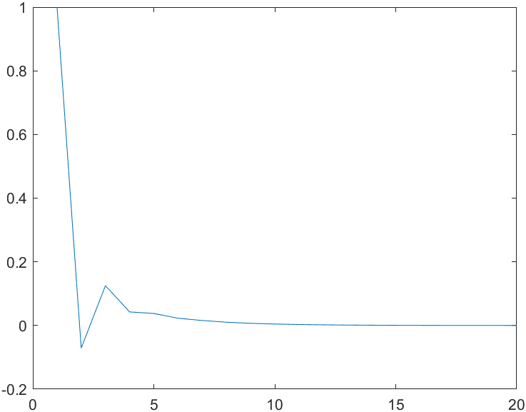
The above is stable, but the projection theorem, which should be less conservative, is unstable, as follows.
Projective singular system (mu=[1;1])
solution =

  With the following fields struct:

    yalmiptime: 0.6001
    solvertime: 0.5069
          info: 'Infeasible problem (MOSEK)'
       problem: 1


++++++++++++++++++++++++++++++++++++++++++++++++++++++++++++++++++++++++++++++++
|   ID|               Constraint|   Primal residual|   Dual residual|       Tag|
++++++++++++++++++++++++++++++++++++++++++++++++++++++++++++++++++++++++++++++++
|   #1|   Elementwise inequality|            1.0041|      4.0782e-15|   gamma_d|
|   #2|        Matrix inequality|        6.5689e-13|      6.5265e-13|         P|
|   #3|        Matrix inequality|          -0.14899|      5.7875e-13|     LMI_S|
++++++++++++++++++++++++++++++++++++++++++++++++++++++++++++++++++++++++++++++++


gamma =

    1.0041


GG =

    0.2874


GGKK =

   3.4754e-07


K =

   1.2093e-06


A =

    1.0000    0.4000
    0.8000    0.9000


ans =

    1.5179
    0.3821


AA =

    1.0000    0.4000
    0.8000    0.9000


ans =

    1.5179
    0.3821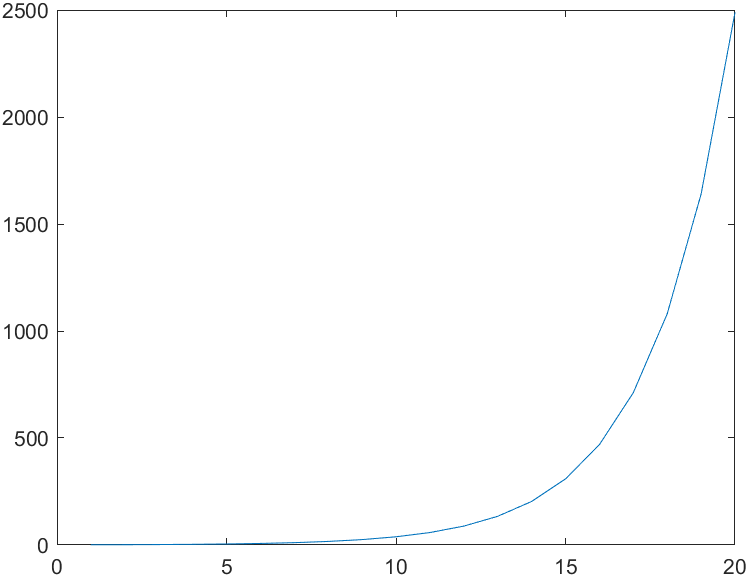
(mu=[1;0])
solution =

  With the following fields struct:

    yalmiptime: 0.5623
    solvertime: 0.4857
          info: 'Numerical problems (MOSEK)'
       problem: 4


++++++++++++++++++++++++++++++++++++++++++++++++++++++++++++++++++++++++++++++++
|   ID|               Constraint|   Primal residual|   Dual residual|       Tag|
++++++++++++++++++++++++++++++++++++++++++++++++++++++++++++++++++++++++++++++++
|   #1|   Elementwise inequality|   2482340499.1025|        -0.15817|   gamma_d|
|   #2|        Matrix inequality|          -0.10809|   43297719.4095|         P|
|   #3|        Matrix inequality|          -0.45821|         0.47314|     LMI_S|
++++++++++++++++++++++++++++++++++++++++++++++++++++++++++++++++++++++++++++++++


gamma =

   2.4823e+09


GG =

    2.3926


GGKK =

   -2.4007


K =

   -1.0034


A =

    1.0000    0.4000
    0.8000    0.9000


ans =

    1.5179
    0.3821


AA =

   -0.0034    0.4000
   -0.2034    0.9000


ans =

    0.0981
    0.7986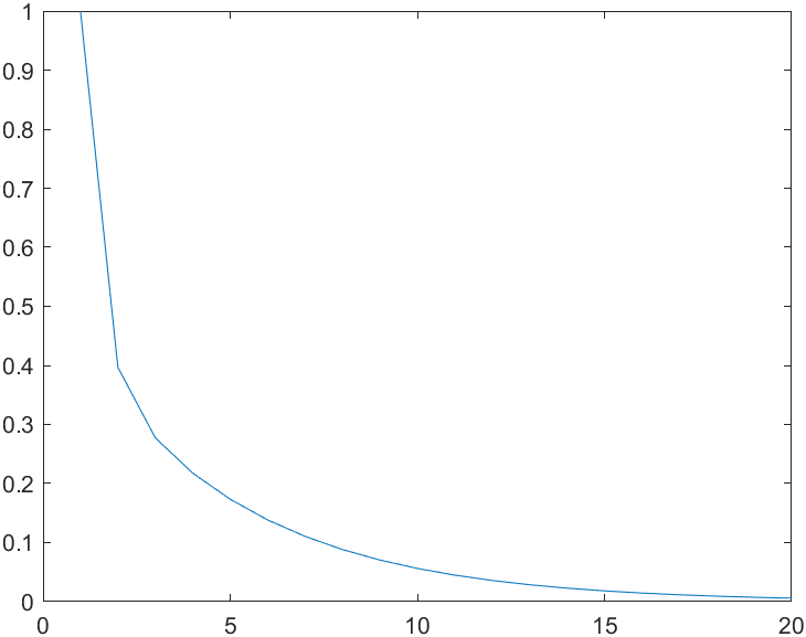
(mu=[0;1])
solution =

  With the following fields struct:

    yalmiptime: 0.6541
    solvertime: 0.4359
          info: 'Infeasible problem (MOSEK)'
       problem: 1


++++++++++++++++++++++++++++++++++++++++++++++++++++++++++++++++++++++++++++++++
|   ID|               Constraint|   Primal residual|   Dual residual|       Tag|
++++++++++++++++++++++++++++++++++++++++++++++++++++++++++++++++++++++++++++++++
|   #1|   Elementwise inequality|            1.1558|      -1.973e-15|   gamma_d|
|   #2|        Matrix inequality|       -1.1323e-15|       0.0040334|         P|
|   #3|        Matrix inequality|          -0.17133|       2.644e-15|     LMI_S|
++++++++++++++++++++++++++++++++++++++++++++++++++++++++++++++++++++++++++++++++


gamma =

    1.1558


GG =

   4.8862e-15


GGKK =

   1.6832e-14


K =

    3.4448


A =

    1.0000    0.4000
    0.8000    0.9000


ans =

    1.5179
    0.3821


AA =

    4.4448    0.4000
    4.2448    0.9000


ans =

    4.8722
    0.4726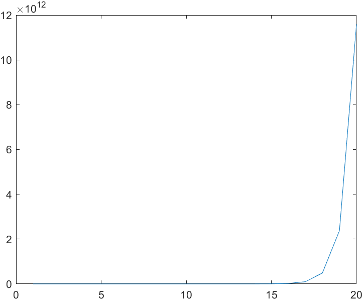
To sum up, it may be that the example is not good and it is difficult to distinguish the two methods. What puzzles me is why there is such a big difference in the controller gain between the two. I need to find an example that is unstable but has a solution with these two methods.
I looked for quite a lot and found: is the quadratic Lyapunov of horizontal slot and output feedback so difficult to stabilize?
So I want to try the output feedback with memory.
Memory output feedback
Without considering event triggering, memory can be understood as:... If you want to use a singular system, it's a little complicated. Forget it.
In fact, state feedback can be directly considered.
state feedback
A little change should do.
Shur complement nonsingular program
clear all;yalmip('clear');

A=[1 0.05;-1.3125 1];B=[0;0.5357];C1=[1 0];D1=[0.1;0];C2=[0.1 0.2];D2=[0];

[n_y,n_x]=size(C1);
n_d=1;
theta=6.0490e-12;
gamma_2=sdpvar(1,1,'full');
P=sdpvar(n_x,n_x);
Y=sdpvar(n_d,n_d);
G=sdpvar(n_d,n_x);

Q=[-P              zeros(n_x,n_d)    (P*A+B*G)'  C2'           ;
    zeros(n_d,n_x) -gamma_2*eye(n_d) (P*D1)'        D2'           ;
    (P*A+B*G)   (P*D1)            -P             zeros(n_x,n_d);
    C2             D2                zeros(n_d,n_x) -eye(n_d)    ];

Theta=[-theta*eye(n_d) (P*B-B*Y)';
    (P*B-B*Y) -eye(n_x)];

LMI_S= [lmi(gamma_2>=0):'gamma_2'];
LMI_S= LMI_S+[lmi(P>=0):'P'];
LMI_S= LMI_S+[lmi(Q<=0):'Q'];


options = sdpsettings('solver','mosek','shift','0.00');
solution = optimize(LMI_S, gamma_2,options)
check(LMI_S)

gamma_2= sqrt(value(gamma_2))

GG=value(G)
YY=value(Y)
K=YY'*GG
A
eig(A)
AA=A+B*K
eig(AA)

x=[1;1];
for i=1:1:20
    X(:,i)=x;
    x=AA*x;
end
plot(X(1,:))