Convolutional Neural Network
Experimental environment
keras 2.1.5
tensorflow 1.4.0
Experimental tools
Jupyter Notebook
Experiment 1: Handwritten Number Classification
Experimental purpose
Grayscale images of handwritten numbers (28 pixels by 28 pixels) are classified into 10 categories (0 to 9).
data set
MNIST dataset:
MNIST dataset is a classic dataset in the field of machine learning.This is a set of 60,000 training images plus 10,000 test images developed by the National Institute of Standards and Technology (NIST) in the 1980s.You can think of solving MNIST classification problems as Hello World for in-depth learning.
Experimental process
1. Basic structure of convolution neural networks:
It is a series of two-dimensional convolution layers and two-dimensional maximum pooling layers.
Importantly, a convolution network requires input of shapeful tensors (image height, image width, image channel) (excluding the dimension of batch processing).In this example, the input of the convolution network processing size (28,28,1) will be set, which is the format of the mnist image.We do this by transferring the parameter input_shape=(28, 28, 1) to the first layer.
from keras import layers
from keras import models

model = models.Sequential()
model.add(layers.Conv2D(32, (3, 3), activation='relu', input_shape=(28, 28, 1)))
model.add(layers.MaxPooling2D((2, 2)))
model.add(layers.Conv2D(64, (3, 3), activation='relu'))
model.add(layers.MaxPooling2D((2, 2)))
model.add(layers.Conv2D(64, (3, 3), activation='relu'))
2. Specific architecture of convolution network:
model.summary()
'''
_________________________________________________________________
Layer (type)                 Output Shape              Param #
=================================================================
conv2d_1 (Conv2D)            (None, 26, 26, 32)        320
_________________________________________________________________
max_pooling2d_1 (MaxPooling2 (None, 13, 13, 32)        0
_________________________________________________________________
conv2d_2 (Conv2D)            (None, 11, 11, 64)        18496
_________________________________________________________________
max_pooling2d_2 (MaxPooling2 (None, 5, 5, 64)          0
_________________________________________________________________
conv2d_3 (Conv2D)            (None, 3, 3, 64)          36928
=================================================================
Total params: 55,744
Trainable params: 55,744
Non-trainable params: 0
_________________________________________________________________
'''
#The output of each two-dimensional convolution layer and the two-dimensional maximum pooled layer is a three-dimensional shape tensor (height, width, number of channels).As the network goes deeper, the width and height shrink.The number of channels passed from one to two dimensions
#The first parameter control of the convolution layer (for example, 32 or 64).
3. Enter our last output tensor (shape (3,3,64)) into a densely connected classification network:
These classifiers deal with vectors that are one-dimensional, and our output now is a three-dimensional tensor.Therefore, first we flatten the three-dimensional output to one dimension, then add some dense layers at the top:
model.add(layers.Flatten())
model.add(layers.Dense(64, activation='relu'))
model.add(layers.Dense(10, activation='softmax'))

model.summary()
'''
_________________________________________________________________
Layer (type)                 Output Shape              Param #
=================================================================
conv2d_1 (Conv2D)            (None, 26, 26, 32)        320
_________________________________________________________________
max_pooling2d_1 (MaxPooling2 (None, 13, 13, 32)        0
_________________________________________________________________
conv2d_2 (Conv2D)            (None, 11, 11, 64)        18496
_________________________________________________________________
max_pooling2d_2 (MaxPooling2 (None, 5, 5, 64)          0
_________________________________________________________________
conv2d_3 (Conv2D)            (None, 3, 3, 64)          36928
_________________________________________________________________
flatten_1 (Flatten)          (None, 576)               0
_________________________________________________________________
dense_1 (Dense)              (None, 64)                36928
_________________________________________________________________
dense_2 (Dense)              (None, 10)                650
=================================================================
Total params: 93,322
Trainable params: 93,322
Non-trainable params: 0
_________________________________________________________________
'''
4. Training:
from keras.datasets import mnist
from keras.utils import to_categorical

(train_images, train_labels), (test_images, test_labels) = mnist.load_data()

train_images = train_images.reshape((60000, 28, 28, 1))
train_images = train_images.astype('float32') / 255

test_images = test_images.reshape((10000, 28, 28, 1))
test_images = test_images.astype('float32') / 255

train_labels = to_categorical(train_labels)
test_labels = to_categorical(test_labels)

model.compile(optimizer='rmsprop',
              loss='categorical_crossentropy',
              metrics=['accuracy'])
model.fit(train_images, train_labels, epochs=5, batch_size=64)
'''
Epoch 1/5
60000/60000 [==============================] - 160s 3ms/step - loss: 0.1797 - acc: 0.9438
Epoch 2/5
60000/60000 [==============================] - 163s 3ms/step - loss: 0.0474 - acc: 0.9857
Epoch 3/5
60000/60000 [==============================] - 8673s 145ms/step - loss: 0.0327 - acc: 0.9896
Epoch 4/5
60000/60000 [==============================] - 39s 647us/step - loss: 0.0248 - acc: 0.9924
Epoch 5/5
60000/60000 [==============================] - 37s 615us/step - loss: 0.0196 - acc: 0.9942

<keras.callbacks.History at 0x1fac5e8cf60>
'''
5. Assessment:
test_loss, test_acc = model.evaluate(test_images, test_labels)
'''
10000/10000 [==============================] - 3s 255us/step
'''
test_acc
'''
0.99019999999999997
'''
#The test accuracy reached an astonishing 99.1%.
Code Integration
from keras import layers
from keras import models

model = models.Sequential()
model.add(layers.Conv2D(32, (3, 3), activation='relu', input_shape=(28, 28, 1)))
model.add(layers.MaxPooling2D((2, 2)))
model.add(layers.Conv2D(64, (3, 3), activation='relu'))
model.add(layers.MaxPooling2D((2, 2)))
model.add(layers.Conv2D(64, (3, 3), activation='relu'))

model.summary()

model.add(layers.Flatten())
model.add(layers.Dense(64, activation='relu'))
model.add(layers.Dense(10, activation='softmax'))

model.summary()

from keras.datasets import mnist
from keras.utils import to_categorical

(train_images, train_labels), (test_images, test_labels) = mnist.load_data()

train_images = train_images.reshape((60000, 28, 28, 1))
train_images = train_images.astype('float32') / 255

test_images = test_images.reshape((10000, 28, 28, 1))
test_images = test_images.astype('float32') / 255

train_labels = to_categorical(train_labels)
test_labels = to_categorical(test_labels)

model.compile(optimizer='rmsprop',
              loss='categorical_crossentropy',
              metrics=['accuracy'])
model.fit(train_images, train_labels, epochs=5, batch_size=64)

test_loss, test_acc = model.evaluate(test_images, test_labels)

test_acc
Experiment 2: Convolutional neural networks using small datasets
Experimental purpose
In a dataset containing 4,000 images of cats and dogs (2,000 cats and 2,000 dogs), the images were classified as "dog" or "cat".
data set
Cat and Dog Dataset:
This original dataset contains 25,000 images of dogs and cats (12,500 per course) and is 543 MB in size (compressed).After downloading and decompressing, we will create a new dataset with three subsets: a training set of 1000 samples per class, a validation set of 500 samples per class, and a test set of 500 samples per class.
Experimental process
1. Download the dataset:
Create a new dataset that contains three subsets: a training set of 1000 samples per class, a validation set of 500 samples per class, and a test set of 500 samples per class.
import os, shutil

original_dataset_dir = 'kaggle_original_data/train'

# The directory where we will
# store our smaller dataset
base_dir = 'cats_and_dogs_small'
os.mkdir(base_dir)

train_dir = os.path.join(base_dir, 'train')
os.mkdir(train_dir)
validation_dir = os.path.join(base_dir, 'validation')
os.mkdir(validation_dir)
test_dir = os.path.join(base_dir, 'test')
os.mkdir(test_dir)

train_cats_dir = os.path.join(train_dir, 'cats')
os.mkdir(train_cats_dir)
train_dogs_dir = os.path.join(train_dir, 'dogs')
os.mkdir(train_dogs_dir)
validation_cats_dir = os.path.join(validation_dir, 'cats')
os.mkdir(validation_cats_dir)
validation_dogs_dir = os.path.join(validation_dir, 'dogs')
os.mkdir(validation_dogs_dir)
test_cats_dir = os.path.join(test_dir, 'cats')
os.mkdir(test_cats_dir)
test_dogs_dir = os.path.join(test_dir, 'dogs')
os.mkdir(test_dogs_dir)

#
fnames = ['cat.{}.jpg'.format(i) for i in range(1000)]
for fname in fnames:
    src = os.path.join(original_dataset_dir, fname)
    dst = os.path.join(train_cats_dir, fname)
    shutil.copyfile(src, dst)

# Copy next 500 cat images to validation_cats_dir
fnames = ['cat.{}.jpg'.format(i) for i in range(1000, 1500)]
for fname in fnames:
    src = os.path.join(original_dataset_dir, fname)
    dst = os.path.join(validation_cats_dir, fname)
    shutil.copyfile(src, dst)

# Copy next 500 cat images to test_cats_dir
fnames = ['cat.{}.jpg'.format(i) for i in range(1500, 2000)]
for fname in fnames:
    src = os.path.join(original_dataset_dir, fname)
    dst = os.path.join(test_cats_dir, fname)
    shutil.copyfile(src, dst)

# Copy first 1000 dog images to train_dogs_dir
fnames = ['dog.{}.jpg'.format(i) for i in range(1000)]
for fname in fnames:
    src = os.path.join(original_dataset_dir, fname)
    dst = os.path.join(train_dogs_dir, fname)
    shutil.copyfile(src, dst)

# Copy next 500 dog images to validation_dogs_dir
fnames = ['dog.{}.jpg'.format(i) for i in range(1000, 1500)]
for fname in fnames:
    src = os.path.join(original_dataset_dir, fname)
    dst = os.path.join(validation_dogs_dir, fname)
    shutil.copyfile(src, dst)

# Copy next 500 dog images to test_dogs_dir
fnames = ['dog.{}.jpg'.format(i) for i in range(1500, 2000)]
for fname in fnames:
    src = os.path.join(original_dataset_dir, fname)
    dst = os.path.join(test_dogs_dir, fname)
    shutil.copyfile(src, dst)

print('total training cat images:', len(os.listdir(train_cats_dir)))
'''
total training cat images: 1000
'''
print('total training dog images:', len(os.listdir(train_dogs_dir)))
'''
total training dog images: 1000
'''
print('total validation cat images:', len(os.listdir(validation_cats_dir)))
'''
total validation cat images: 500
'''
print('total validation dog images:', len(os.listdir(validation_dogs_dir)))
'''
total validation dog images: 500
'''
print('total test cat images:', len(os.listdir(test_cats_dir)))
'''
total test cat images: 500
'''
print('total test dog images:', len(os.listdir(test_dogs_dir)))
'''
total test dog images: 500
'''
2. Set up a network:
Our convolution network is a stack of alternating Conv2D (with Relu activation) and Max pooled 2D layers, which will have a Conv2D + MaxPooling 2D phase and a single cell (full-connected layer of size 1) and a S-shape activation as network output layers to handle larger images and more complex problems.
from keras import layers
from keras import models

model = models.Sequential()
model.add(layers.Conv2D(32, (3, 3), activation='relu',
                        input_shape=(150, 150, 3)))
model.add(layers.MaxPooling2D((2, 2)))
model.add(layers.Conv2D(64, (3, 3), activation='relu'))
model.add(layers.MaxPooling2D((2, 2)))
model.add(layers.Conv2D(128, (3, 3), activation='relu'))
model.add(layers.MaxPooling2D((2, 2)))
model.add(layers.Conv2D(128, (3, 3), activation='relu'))
model.add(layers.MaxPooling2D((2, 2)))
model.add(layers.Flatten())
model.add(layers.Dense(512, activation='relu'))
model.add(layers.Dense(1, activation='sigmoid'))

model.summary()
'''
_________________________________________________________________
Layer (type)                 Output Shape              Param #
=================================================================
conv2d_1 (Conv2D)            (None, 148, 148, 32)      896
_________________________________________________________________
max_pooling2d_1 (MaxPooling2 (None, 74, 74, 32)        0
_________________________________________________________________
conv2d_2 (Conv2D)            (None, 72, 72, 64)        18496
_________________________________________________________________
max_pooling2d_2 (MaxPooling2 (None, 36, 36, 64)        0
_________________________________________________________________
conv2d_3 (Conv2D)            (None, 34, 34, 128)       73856
_________________________________________________________________
max_pooling2d_3 (MaxPooling2 (None, 17, 17, 128)       0
_________________________________________________________________
conv2d_4 (Conv2D)            (None, 15, 15, 128)       147584
_________________________________________________________________
max_pooling2d_4 (MaxPooling2 (None, 7, 7, 128)         0
_________________________________________________________________
flatten_1 (Flatten)          (None, 6272)              0
_________________________________________________________________
dense_1 (Dense)              (None, 512)               3211776
_________________________________________________________________
dense_2 (Dense)              (None, 1)                 513
=================================================================
Total params: 3,453,121
Trainable params: 3,453,121
Non-trainable params: 0
_________________________________________________________________
'''
Using RMSprop optimizer:
Since the output layer of the network is a single simoid cell, the binary cross-entropy is used as our loss function.
from keras import optimizers

model.compile(loss='binary_crossentropy',
              optimizer=optimizers.RMSprop(lr=1e-4),
              metrics=['acc'])
4. Data preprocessing:
Preprocessed floating-point tensors should be used to format data before entering our network.
The steps to import it into our network are as follows:
1. Read picture files
2. Decode JPEG content into a RBG grid of pixels.
3. Convert these to floating-point tensors.
4. Rescale the pixel values (between 0 and 255) to [0,1] intervals (as you know, neural networks tend to handle small input values).
from keras.preprocessing.image import ImageDataGenerator

# All images will be rescaled by 1./255
train_datagen = ImageDataGenerator(rescale=1./255)
test_datagen = ImageDataGenerator(rescale=1./255)

train_generator = train_datagen.flow_from_directory(
        # This is the target directory
        train_dir,
        # All images will be resized to 150x150
        target_size=(150, 150),
        batch_size=20,
        # Since we use binary_crossentropy loss, we need binary labels
        class_mode='binary')

validation_generator = test_datagen.flow_from_directory(
        validation_dir,
        target_size=(150, 150),
        batch_size=20,
        class_mode='binary')
'''
Found 2000 images belonging to 2 classes.
Found 1000 images belonging to 2 classes.
'''
#View the output of one of the generators:
#It produces batches of 150x150 RGB images (shapes (20,150,150,3)) and binary labels (shapes (20,)).20 is the number of samples in each batch (batch size).
for data_batch, labels_batch in train_generator:
    print('data batch shape:', data_batch.shape)
    print('labels batch shape:', labels_batch.shape)
    break
'''
data batch shape: (20, 150, 150, 3)
labels batch shape: (20,)
'''
5. Fitting:
Using the Fit Generator method.
history = model.fit_generator(
      train_generator,
      steps_per_epoch=100,
      epochs=30,
      validation_data=validation_generator,
      validation_steps=50)
'''
Epoch 1/30
100/100 [==============================] - 1269s 13s/step - loss: 0.6859 - acc: 0.5475 - val_loss: 0.6616 - val_acc: 0.6420
Epoch 2/30
100/100 [==============================] - 27s 269ms/step - loss: 0.6353 - acc: 0.6390 - val_loss: 0.6266 - val_acc: 0.6590
Epoch 3/30
100/100 [==============================] - 24s 237ms/step - loss: 0.5914 - acc: 0.6910 - val_loss: 0.6410 - val_acc: 0.6390
Epoch 4/30
100/100 [==============================] - 24s 240ms/step - loss: 0.5601 - acc: 0.7165 - val_loss: 0.6574 - val_acc: 0.6340
Epoch 5/30
100/100 [==============================] - 25s 248ms/step - loss: 0.5373 - acc: 0.7265 - val_loss: 0.6056 - val_acc: 0.6720
Epoch 6/30
100/100 [==============================] - 20s 195ms/step - loss: 0.5116 - acc: 0.7505 - val_loss: 0.5675 - val_acc: 0.6990
Epoch 7/30
100/100 [==============================] - 20s 196ms/step - loss: 0.4860 - acc: 0.7560 - val_loss: 0.5564 - val_acc: 0.6980
Epoch 8/30
100/100 [==============================] - 20s 202ms/step - loss: 0.4555 - acc: 0.7840 - val_loss: 0.5694 - val_acc: 0.7020
Epoch 9/30
100/100 [==============================] - 23s 233ms/step - loss: 0.4339 - acc: 0.7990 - val_loss: 0.5547 - val_acc: 0.7100
Epoch 10/30
100/100 [==============================] - 21s 208ms/step - loss: 0.4034 - acc: 0.8185 - val_loss: 0.5484 - val_acc: 0.7280
Epoch 11/30
100/100 [==============================] - 22s 217ms/step - loss: 0.3810 - acc: 0.8295 - val_loss: 0.5737 - val_acc: 0.7220
Epoch 12/30
100/100 [==============================] - 22s 218ms/step - loss: 0.3609 - acc: 0.8455 - val_loss: 0.6161 - val_acc: 0.7010
Epoch 13/30
100/100 [==============================] - 21s 208ms/step - loss: 0.3415 - acc: 0.8470 - val_loss: 0.5498 - val_acc: 0.7260
Epoch 14/30
100/100 [==============================] - 20s 205ms/step - loss: 0.3190 - acc: 0.8640 - val_loss: 0.5676 - val_acc: 0.7250
Epoch 15/30
100/100 [==============================] - 20s 204ms/step - loss: 0.2891 - acc: 0.8865 - val_loss: 0.5854 - val_acc: 0.7420
Epoch 16/30
100/100 [==============================] - 21s 205ms/step - loss: 0.2694 - acc: 0.8890 - val_loss: 0.5864 - val_acc: 0.7290
Epoch 17/30
100/100 [==============================] - 20s 203ms/step - loss: 0.2471 - acc: 0.9015 - val_loss: 0.6189 - val_acc: 0.7210
Epoch 18/30
100/100 [==============================] - 25s 248ms/step - loss: 0.2318 - acc: 0.9105 - val_loss: 0.6030 - val_acc: 0.7300
Epoch 19/30
100/100 [==============================] - 23s 227ms/step - loss: 0.2075 - acc: 0.9220 - val_loss: 0.8091 - val_acc: 0.6860
Epoch 20/30
100/100 [==============================] - 24s 236ms/step - loss: 0.1872 - acc: 0.9350 - val_loss: 0.6385 - val_acc: 0.7480
Epoch 21/30
100/100 [==============================] - 22s 220ms/step - loss: 0.1730 - acc: 0.9435 - val_loss: 0.6707 - val_acc: 0.7330
Epoch 22/30
100/100 [==============================] - 27s 267ms/step - loss: 0.1569 - acc: 0.9465 - val_loss: 0.6582 - val_acc: 0.7440
Epoch 23/30
100/100 [==============================] - 25s 246ms/step - loss: 0.1438 - acc: 0.9485 - val_loss: 0.6917 - val_acc: 0.7460
Epoch 24/30
100/100 [==============================] - 28s 284ms/step - loss: 0.1239 - acc: 0.9585 - val_loss: 0.7309 - val_acc: 0.7400
Epoch 25/30
100/100 [==============================] - 24s 245ms/step - loss: 0.1099 - acc: 0.9625 - val_loss: 0.7476 - val_acc: 0.7290
Epoch 26/30
100/100 [==============================] - 25s 248ms/step - loss: 0.0936 - acc: 0.9700 - val_loss: 0.7722 - val_acc: 0.7390
Epoch 27/30
100/100 [==============================] - 21s 210ms/step - loss: 0.0811 - acc: 0.9740 - val_loss: 1.1478 - val_acc: 0.6940
Epoch 28/30
100/100 [==============================] - 21s 209ms/step - loss: 0.0717 - acc: 0.9780 - val_loss: 0.9114 - val_acc: 0.7130
Epoch 29/30
100/100 [==============================] - 21s 214ms/step - loss: 0.0634 - acc: 0.9800 - val_loss: 0.8197 - val_acc: 0.7400
Epoch 30/30
100/100 [==============================] - 22s 218ms/step - loss: 0.0561 - acc: 0.9840 - val_loss: 0.8574 - val_acc: 0.7360
'''
#Save Model
model.save('cats_and_dogs_small_1.h5')
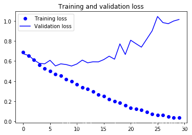
6. Draw the loss function and accuracy in the training and validation sets:
Overfitting occurred.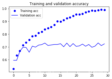
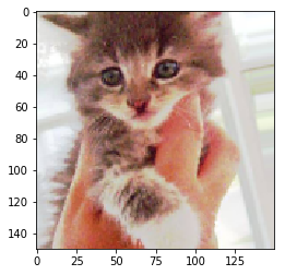
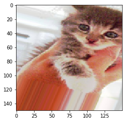
7. Data Enhancement:
Fitting is caused by not having too many samples to learn, which prevents us from training models that can be extended to new data.Given unlimited data, our model will cover every possible aspect of the distribution of the data at hand: we will never overuse it.Data enhancement uses the method of generating more training data from existing training samples and "enhances" the samples through some random transformations to produce reliable images.The goal is that during training, our model will never see the exact same picture again.This helps the model to cover more aspects of the data and to be more generalized.
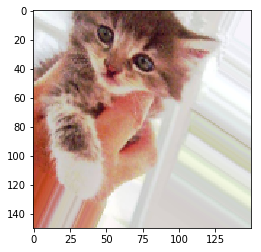
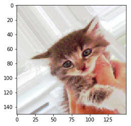
#Configure a large number of random transformations
datagen = ImageDataGenerator(
      rotation_range=40,       #Randomly rotate the range of the picture
      width_shift_range=0.2,   #Randomly transform the range of the picture vertically or horizontally
      height_shift_range=0.2,
      shear_range=0.2,         #Random application of shear transformation
      zoom_range=0.2,          #Random zoom of internal photos
      horizontal_flip=True,    #Flip half of the image horizontally and randomly
      fill_mode='nearest')     #Used to populate newly created pixels

#View enhanced images
from keras.preprocessing import image
fnames = [os.path.join(train_cats_dir, fname) for fname in os.listdir(train_cats_dir)]
img_path = fnames[3]
img = image.load_img(img_path, target_size=(150, 150))
x = image.img_to_array(img)
x = x.reshape((1,) + x.shape)
i = 0
for batch in datagen.flow(x, batch_size=1):
    plt.figure(i)
    imgplot = plt.imshow(image.array_to_img(batch[0]))
    i += 1
    if i % 4 == 0:
        break
plt.show()
Inputs are still heavily correlated, so this may not be enough to get rid of fit completely.To further solve the fitting problem, we will also add a Dropout layer to the model before densely connected classifiers:
model = models.Sequential()
model.add(layers.Conv2D(32, (3, 3), activation='relu',
                        input_shape=(150, 150, 3)))
model.add(layers.MaxPooling2D((2, 2)))
model.add(layers.Conv2D(64, (3, 3), activation='relu'))
model.add(layers.MaxPooling2D((2, 2)))
model.add(layers.Conv2D(128, (3, 3), activation='relu'))
model.add(layers.MaxPooling2D((2, 2)))
model.add(layers.Conv2D(128, (3, 3), activation='relu'))
model.add(layers.MaxPooling2D((2, 2)))
model.add(layers.Flatten())
model.add(layers.Dropout(0.5))
model.add(layers.Dense(512, activation='relu'))
model.add(layers.Dense(1, activation='sigmoid'))

model.compile(loss='binary_crossentropy',
              optimizer=optimizers.RMSprop(lr=1e-4),
              metrics=['acc'])
8. Training network:
train_datagen = ImageDataGenerator(
    rescale=1./255,
    rotation_range=40,
    width_shift_range=0.2,
    height_shift_range=0.2,
    shear_range=0.2,
    zoom_range=0.2,
    horizontal_flip=True,)

# Note that the validation data should not be augmented!
test_datagen = ImageDataGenerator(rescale=1./255)

train_generator = train_datagen.flow_from_directory(
        # This is the target directory
        train_dir,
        # All images will be resized to 150x150
        target_size=(150, 150),
        batch_size=32,
        # Since we use binary_crossentropy loss, we need binary labels
        class_mode='binary')

validation_generator = test_datagen.flow_from_directory(
        validation_dir,
        target_size=(150, 150),
        batch_size=32,
        class_mode='binary')

history = model.fit_generator(
      train_generator,
      steps_per_epoch=100,
      epochs=10,
      validation_data=validation_generator,
      validation_steps=50)
'''
Found 2000 images belonging to 2 classes.
Found 1000 images belonging to 2 classes.
Epoch 1/10
100/100 [==============================] - 65s 646ms/step - loss: 0.6938 - acc: 0.5212 - val_loss: 0.6851 - val_acc: 0.4956
Epoch 2/10
100/100 [==============================] - 57s 574ms/step - loss: 0.6838 - acc: 0.5513 - val_loss: 0.6942 - val_acc: 0.5089
Epoch 3/10
100/100 [==============================] - 57s 573ms/step - loss: 0.6700 - acc: 0.5828 - val_loss: 0.6439 - val_acc: 0.6136
Epoch 4/10
100/100 [==============================] - 57s 571ms/step - loss: 0.6478 - acc: 0.6275 - val_loss: 0.6255 - val_acc: 0.6225
Epoch 5/10
100/100 [==============================] - 59s 586ms/step - loss: 0.6324 - acc: 0.6428 - val_loss: 0.5974 - val_acc: 0.6834
Epoch 6/10
100/100 [==============================] - 60s 604ms/step - loss: 0.6126 - acc: 0.6678 - val_loss: 0.5896 - val_acc: 0.6593
Epoch 7/10
100/100 [==============================] - 66s 662ms/step - loss: 0.6132 - acc: 0.6597 - val_loss: 0.5620 - val_acc: 0.7164
Epoch 8/10
100/100 [==============================] - 57s 572ms/step - loss: 0.6044 - acc: 0.6672 - val_loss: 0.5758 - val_acc: 0.6872
Epoch 9/10
100/100 [==============================] - 76s 764ms/step - loss: 0.5782 - acc: 0.7094 - val_loss: 0.7336 - val_acc: 0.6148
Epoch 10/10
100/100 [==============================] - 87s 866ms/step - loss: 0.5931 - acc: 0.6788 - val_loss: 0.5397 - val_acc: 0.7253
'''
model.save('cats_and_dogs_small_2-10.h5')
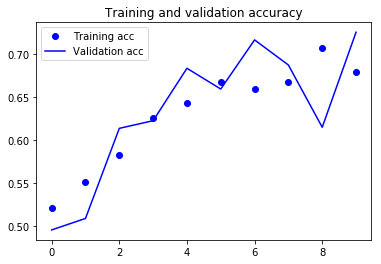
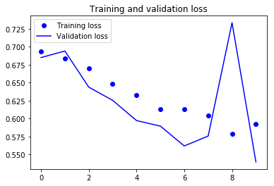
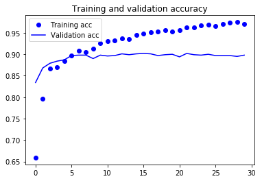
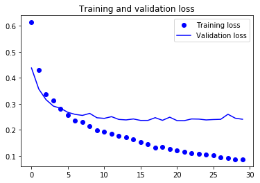
9. Draw the result:
Due to data enhancement and discard strategies, we no longer overfit
acc = history.history['acc']
val_acc = history.history['val_acc']
loss = history.history['loss']
val_loss = history.history['val_loss']

epochs = range(len(acc))

plt.plot(epochs, acc, 'bo', label='Training acc')
plt.plot(epochs, val_acc, 'b', label='Validation acc')
plt.title('Training and validation accuracy')
plt.legend()

plt.figure()

plt.plot(epochs, loss, 'bo', label='Training loss')
plt.plot(epochs, val_loss, 'b', label='Validation loss')
plt.title('Training and validation loss')
plt.legend()

plt.show()
Code Integration
import keras
keras.__version__
import os, shutil

original_dataset_dir = 'kaggle_original_data/train'
base_dir = 'cats_and_dogs_small'
os.mkdir(base_dir)
train_dir = os.path.join(base_dir, 'train')
os.mkdir(train_dir)
validation_dir = os.path.join(base_dir, 'validation')
os.mkdir(validation_dir)
test_dir = os.path.join(base_dir, 'test')
os.mkdir(test_dir)
train_cats_dir = os.path.join(train_dir, 'cats')
os.mkdir(train_cats_dir)
train_dogs_dir = os.path.join(train_dir, 'dogs')
os.mkdir(train_dogs_dir)
validation_cats_dir = os.path.join(validation_dir, 'cats')
os.mkdir(validation_cats_dir)
validation_dogs_dir = os.path.join(validation_dir, 'dogs')
os.mkdir(validation_dogs_dir)
test_cats_dir = os.path.join(test_dir, 'cats')
os.mkdir(test_cats_dir)
test_dogs_dir = os.path.join(test_dir, 'dogs')
os.mkdir(test_dogs_dir)
fnames = ['cat.{}.jpg'.format(i) for i in range(1000)]
for fname in fnames:
    src = os.path.join(original_dataset_dir, fname)
    dst = os.path.join(train_cats_dir, fname)
    shutil.copyfile(src, dst)
fnames = ['cat.{}.jpg'.format(i) for i in range(1000, 1500)]
for fname in fnames:
    src = os.path.join(original_dataset_dir, fname)
    dst = os.path.join(validation_cats_dir, fname)
    shutil.copyfile(src, dst)
fnames = ['cat.{}.jpg'.format(i) for i in range(1500, 2000)]
for fname in fnames:
    src = os.path.join(original_dataset_dir, fname)
    dst = os.path.join(test_cats_dir, fname)
    shutil.copyfile(src, dst)
fnames = ['dog.{}.jpg'.format(i) for i in range(1000)]
for fname in fnames:
    src = os.path.join(original_dataset_dir, fname)
    dst = os.path.join(train_dogs_dir, fname)
    shutil.copyfile(src, dst)
fnames = ['dog.{}.jpg'.format(i) for i in range(1000, 1500)]
for fname in fnames:
    src = os.path.join(original_dataset_dir, fname)
    dst = os.path.join(validation_dogs_dir, fname)
    shutil.copyfile(src, dst)
fnames = ['dog.{}.jpg'.format(i) for i in range(1500, 2000)]
for fname in fnames:
    src = os.path.join(original_dataset_dir, fname)
    dst = os.path.join(test_dogs_dir, fname)
    shutil.copyfile(src, dst)

from keras import layers
from keras import models

model = models.Sequential()
model.add(layers.Conv2D(32, (3, 3), activation='relu',
                        input_shape=(150, 150, 3)))
model.add(layers.MaxPooling2D((2, 2)))
model.add(layers.Conv2D(64, (3, 3), activation='relu'))
model.add(layers.MaxPooling2D((2, 2)))
model.add(layers.Conv2D(128, (3, 3), activation='relu'))
model.add(layers.MaxPooling2D((2, 2)))
model.add(layers.Conv2D(128, (3, 3), activation='relu'))
model.add(layers.MaxPooling2D((2, 2)))
model.add(layers.Flatten())
model.add(layers.Dense(512, activation='relu'))
model.add(layers.Dense(1, activation='sigmoid'))

from keras import optimizers

model.compile(loss='binary_crossentropy',
              optimizer=optimizers.RMSprop(lr=1e-4),
              metrics=['acc'])

from keras.preprocessing.image import ImageDataGenerator

train_datagen = ImageDataGenerator(rescale=1./255)
test_datagen = ImageDataGenerator(rescale=1./255)
train_generator = train_datagen.flow_from_directory(
        train_dir,
        target_size=(150, 150),
        batch_size=20,
        class_mode='binary')
validation_generator = test_datagen.flow_from_directory(
        validation_dir,
        target_size=(150, 150),
        batch_size=20,
        class_mode='binary')

for data_batch, labels_batch in train_generator:
    print('data batch shape:', data_batch.shape)
    print('labels batch shape:', labels_batch.shape)
    break

history = model.fit_generator(
      train_generator,
      steps_per_epoch=100,
      epochs=30,
      validation_data=validation_generator,
      validation_steps=50)

datagen = ImageDataGenerator(
      rotation_range=40,
      width_shift_range=0.2,
      height_shift_range=0.2,
      shear_range=0.2,
      zoom_range=0.2,
      horizontal_flip=True,
      fill_mode='nearest')

model = models.Sequential()
model.add(layers.Conv2D(32, (3, 3), activation='relu',
                        input_shape=(150, 150, 3)))
model.add(layers.MaxPooling2D((2, 2)))
model.add(layers.Conv2D(64, (3, 3), activation='relu'))
model.add(layers.MaxPooling2D((2, 2)))
model.add(layers.Conv2D(128, (3, 3), activation='relu'))
model.add(layers.MaxPooling2D((2, 2)))
model.add(layers.Conv2D(128, (3, 3), activation='relu'))
model.add(layers.MaxPooling2D((2, 2)))
model.add(layers.Flatten())
model.add(layers.Dropout(0.5))
model.add(layers.Dense(512, activation='relu'))
model.add(layers.Dense(1, activation='sigmoid'))
model.compile(loss='binary_crossentropy',
              optimizer=optimizers.RMSprop(lr=1e-4),
              metrics=['acc'])

train_datagen = ImageDataGenerator(
    rescale=1./255,
    rotation_range=40,
    width_shift_range=0.2,
    height_shift_range=0.2,
    shear_range=0.2,
    zoom_range=0.2,
    horizontal_flip=True,)

test_datagen = ImageDataGenerator(rescale=1./255)
train_generator = train_datagen.flow_from_directory(
        # This is the target directory
        train_dir,
        # All images will be resized to 150x150
        target_size=(150, 150),
        batch_size=32,
        # Since we use binary_crossentropy loss, we need binary labels
        class_mode='binary')
validation_generator = test_datagen.flow_from_directory(
        validation_dir,
        target_size=(150, 150),
        batch_size=32,
        class_mode='binary')
history = model.fit_generator(
      train_generator,
      steps_per_epoch=100,
      epochs=10,
      validation_data=validation_generator,
      validation_steps=50)

acc = history.history['acc']
val_acc = history.history['val_acc']
loss = history.history['loss']
val_loss = history.history['val_loss']
epochs = range(len(acc))
plt.plot(epochs, acc, 'bo', label='Training acc')
plt.plot(epochs, val_acc, 'b', label='Validation acc')
plt.title('Training and validation accuracy')
plt.legend()
plt.figure()
plt.plot(epochs, loss, 'bo', label='Training loss')
plt.plot(epochs, val_loss, 'b', label='Validation loss')
plt.title('Training and validation loss')
plt.legend()
plt.show()
Experiment 3: Using pre-training convnet
Experimental purpose
Classify ImageNet datasets using the VGG16 architecture.
data set
ImageNet dataset:
ImageNet has 1.4 million tagged images and 1,000 different categories, including many animal categories, including cats and dogs, so you can expect to perform well on our cat and dog classification issues.
Experimental process
There are two ways to effectively utilize the pre-training network: feature extraction and fine-tuning.
feature extraction
Use previously trained networks to extract features of interest from new samples.Then start training from scratch with a new classifier.
1. convnets for image classification consist of two parts: they start with a series of pooling and convolution layers and end with densely connected classifiers.The first part is called the convolution base of the model.For small networks, Feature Extraction simply includes the convolution base of the pre-training network, runs new data through it, and trains a new classifier on top of the output.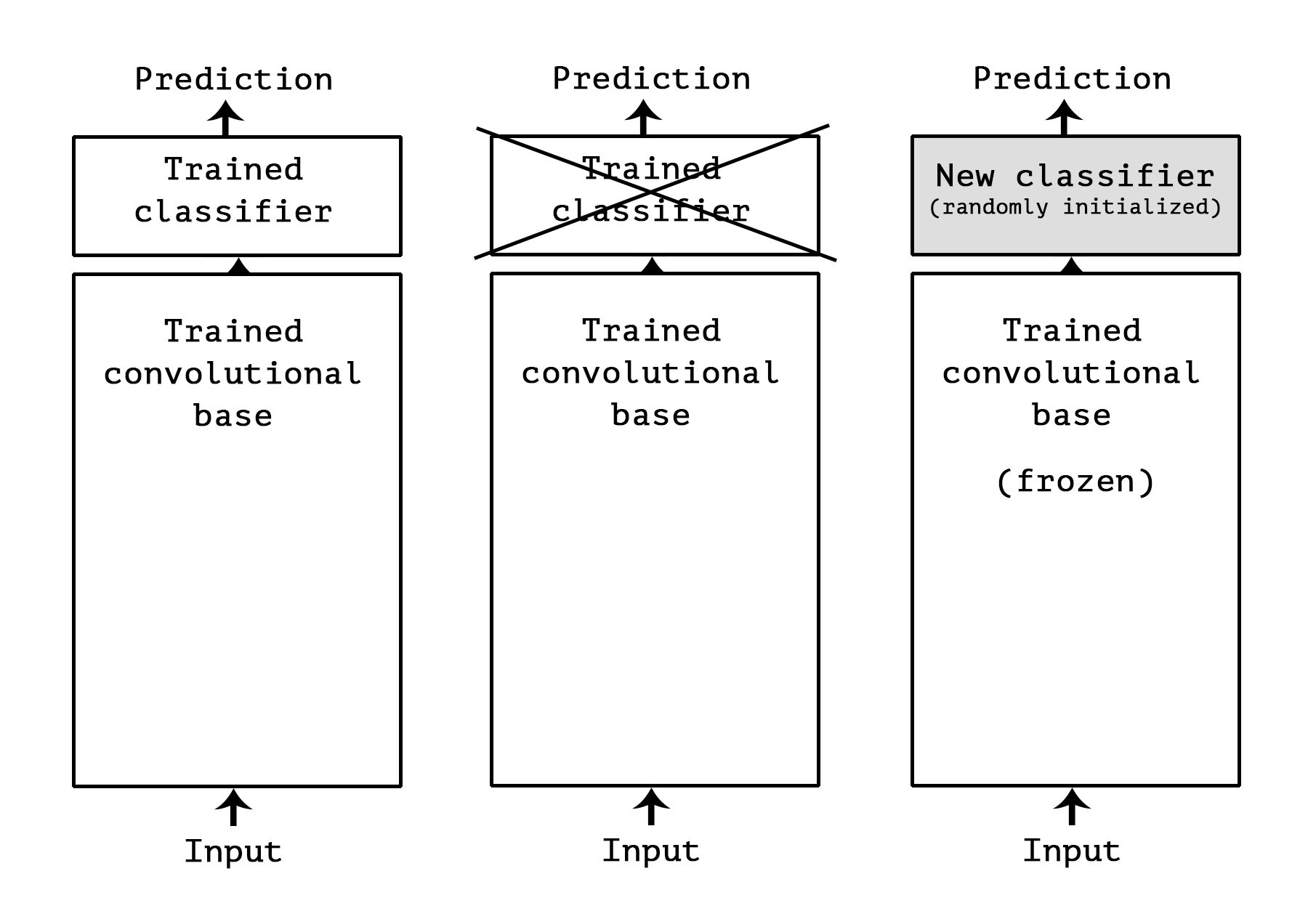
1. Instantiate the VGG16 model:
from keras.applications import VGG16

conv_base = VGG16(weights='imagenet',         #Initial Weight Value
                  include_top=False,          #Is there a densely connected classifier at the top of the network
                  input_shape=(150, 150, 3))  #Shape of the image tensor of the input network

#Details of the VGG16 convolution base architecture
conv_base.summary()
'''
_________________________________________________________________
Layer (type)                 Output Shape              Param #
=================================================================
input_1 (InputLayer)         (None, 150, 150, 3)       0
_________________________________________________________________
block1_conv1 (Conv2D)        (None, 150, 150, 64)      1792
_________________________________________________________________
block1_conv2 (Conv2D)        (None, 150, 150, 64)      36928
_________________________________________________________________
block1_pool (MaxPooling2D)   (None, 75, 75, 64)        0
_________________________________________________________________
block2_conv1 (Conv2D)        (None, 75, 75, 128)       73856
_________________________________________________________________
block2_conv2 (Conv2D)        (None, 75, 75, 128)       147584
_________________________________________________________________
block2_pool (MaxPooling2D)   (None, 37, 37, 128)       0
_________________________________________________________________
block3_conv1 (Conv2D)        (None, 37, 37, 256)       295168
_________________________________________________________________
block3_conv2 (Conv2D)        (None, 37, 37, 256)       590080
_________________________________________________________________
block3_conv3 (Conv2D)        (None, 37, 37, 256)       590080
_________________________________________________________________
block3_pool (MaxPooling2D)   (None, 18, 18, 256)       0
_________________________________________________________________
block4_conv1 (Conv2D)        (None, 18, 18, 512)       1180160
_________________________________________________________________
block4_conv2 (Conv2D)        (None, 18, 18, 512)       2359808
_________________________________________________________________
block4_conv3 (Conv2D)        (None, 18, 18, 512)       2359808
_________________________________________________________________
block4_pool (MaxPooling2D)   (None, 9, 9, 512)         0
_________________________________________________________________
block5_conv1 (Conv2D)        (None, 9, 9, 512)         2359808
_________________________________________________________________
block5_conv2 (Conv2D)        (None, 9, 9, 512)         2359808
_________________________________________________________________
block5_conv3 (Conv2D)        (None, 9, 9, 512)         2359808
_________________________________________________________________
block5_pool (MaxPooling2D)   (None, 4, 4, 512)         0
=================================================================
Total params: 14,714,688
Trainable params: 14,714,688
Non-trainable params: 0
_________________________________________________________________
'''
2. First method:
Run a convolution base on our dataset, save its output to disk as a Numpy array, and use the data as input to a separate densely connected classifier.
import os
import numpy as np
from keras.preprocessing.image import ImageDataGenerator

base_dir = '/Users/Administrator/Desktop/deeplearning/02.Convolutional Neural Network/cats_and_dogs_small'

train_dir = os.path.join(base_dir, 'train')
validation_dir = os.path.join(base_dir, 'validation')
test_dir = os.path.join(base_dir, 'test')

datagen = ImageDataGenerator(rescale=1./255)
batch_size = 20

def extract_features(directory, sample_count):
    features = np.zeros(shape=(sample_count, 4, 4, 512))
    labels = np.zeros(shape=(sample_count))
    generator = datagen.flow_from_directory(
        directory,
        target_size=(150, 150),
        batch_size=batch_size,
        class_mode='binary')
    i = 0
    for inputs_batch, labels_batch in generator:
        features_batch = conv_base.predict(inputs_batch)
        features[i * batch_size : (i + 1) * batch_size] = features_batch
        labels[i * batch_size : (i + 1) * batch_size] = labels_batch
        i += 1
        if i * batch_size >= sample_count:
            # Note that since generators yield data indefinitely in a loop,
            # we must `break` after every image has been seen once.
            break
    return features, labels

train_features, train_labels = extract_features(train_dir, 2000)
validation_features, validation_labels = extract_features(validation_dir, 1000)
test_features, test_labels = extract_features(test_dir, 1000)
'''
Found 2000 images belonging to 2 classes.
Found 1000 images belonging to 2 classes.
Found 1000 images belonging to 2 classes.
'''
#Delayering
train_features = np.reshape(train_features, (2000, 4 * 4 * 512))
validation_features = np.reshape(validation_features, (1000, 4 * 4 * 512))
test_features = np.reshape(test_features, (1000, 4 * 4 * 512))
Training:
Define densely connected classifiers using dropout regularization to train on the data and labels just recorded.
from keras import models
from keras import layers
from keras import optimizers

model = models.Sequential()
model.add(layers.Dense(256, activation='relu', input_dim=4 * 4 * 512))
model.add(layers.Dropout(0.5))
model.add(layers.Dense(1, activation='sigmoid'))

model.compile(optimizer=optimizers.RMSprop(lr=2e-5),
              loss='binary_crossentropy',
              metrics=['acc'])

history = model.fit(train_features, train_labels,
                    epochs=30,
                    batch_size=20,
                    validation_data=(validation_features, validation_labels))
'''
Train on 2000 samples, validate on 1000 samples
Epoch 1/30
2000/2000 [==============================] - 4s 2ms/step - loss: 0.6134 - acc: 0.6590 - val_loss: 0.4378 - val_acc: 0.8340
Epoch 2/30
2000/2000 [==============================] - 4s 2ms/step - loss: 0.4305 - acc: 0.7965 - val_loss: 0.3568 - val_acc: 0.8680
Epoch 3/30
2000/2000 [==============================] - 4s 2ms/step - loss: 0.3378 - acc: 0.8660 - val_loss: 0.3159 - val_acc: 0.8790
Epoch 4/30
2000/2000 [==============================] - 4s 2ms/step - loss: 0.3136 - acc: 0.8705 - val_loss: 0.2912 - val_acc: 0.8840
Epoch 5/30
2000/2000 [==============================] - 4s 2ms/step - loss: 0.2815 - acc: 0.8845 - val_loss: 0.2826 - val_acc: 0.8870
Epoch 6/30
2000/2000 [==============================] - 4s 2ms/step - loss: 0.2578 - acc: 0.8975 - val_loss: 0.2670 - val_acc: 0.8970
Epoch 7/30
2000/2000 [==============================] - 4s 2ms/step - loss: 0.2358 - acc: 0.9075 - val_loss: 0.2592 - val_acc: 0.8980
Epoch 8/30
2000/2000 [==============================] - 4s 2ms/step - loss: 0.2298 - acc: 0.9045 - val_loss: 0.2553 - val_acc: 0.8980
Epoch 9/30
2000/2000 [==============================] - 4s 2ms/step - loss: 0.2144 - acc: 0.9130 - val_loss: 0.2630 - val_acc: 0.8900
Epoch 10/30
2000/2000 [==============================] - 4s 2ms/step - loss: 0.1975 - acc: 0.9255 - val_loss: 0.2461 - val_acc: 0.8980
Epoch 11/30
2000/2000 [==============================] - 4s 2ms/step - loss: 0.1932 - acc: 0.9305 - val_loss: 0.2439 - val_acc: 0.8960
Epoch 12/30
2000/2000 [==============================] - 4s 2ms/step - loss: 0.1832 - acc: 0.9325 - val_loss: 0.2504 - val_acc: 0.8970
Epoch 13/30
2000/2000 [==============================] - 4s 2ms/step - loss: 0.1775 - acc: 0.9370 - val_loss: 0.2398 - val_acc: 0.9010
Epoch 14/30
2000/2000 [==============================] - 4s 2ms/step - loss: 0.1709 - acc: 0.9355 - val_loss: 0.2380 - val_acc: 0.8990
Epoch 15/30
2000/2000 [==============================] - 4s 2ms/step - loss: 0.1644 - acc: 0.9455 - val_loss: 0.2416 - val_acc: 0.9010
Epoch 16/30
2000/2000 [==============================] - 4s 2ms/step - loss: 0.1526 - acc: 0.9485 - val_loss: 0.2359 - val_acc: 0.9020
Epoch 17/30
2000/2000 [==============================] - 4s 2ms/step - loss: 0.1442 - acc: 0.9515 - val_loss: 0.2360 - val_acc: 0.9010
Epoch 18/30
2000/2000 [==============================] - 4s 2ms/step - loss: 0.1320 - acc: 0.9535 - val_loss: 0.2465 - val_acc: 0.8970
Epoch 19/30
2000/2000 [==============================] - 4s 2ms/step - loss: 0.1327 - acc: 0.9555 - val_loss: 0.2363 - val_acc: 0.8990
Epoch 20/30
2000/2000 [==============================] - 4s 2ms/step - loss: 0.1263 - acc: 0.9535 - val_loss: 0.2484 - val_acc: 0.9000
Epoch 21/30
2000/2000 [==============================] - 4s 2ms/step - loss: 0.1210 - acc: 0.9570 - val_loss: 0.2352 - val_acc: 0.8940
Epoch 22/30
2000/2000 [==============================] - 4s 2ms/step - loss: 0.1147 - acc: 0.9620 - val_loss: 0.2351 - val_acc: 0.9020
Epoch 23/30
2000/2000 [==============================] - 4s 2ms/step - loss: 0.1108 - acc: 0.9630 - val_loss: 0.2416 - val_acc: 0.8990
Epoch 24/30
2000/2000 [==============================] - 4s 2ms/step - loss: 0.1070 - acc: 0.9680 - val_loss: 0.2411 - val_acc: 0.8980
Epoch 25/30
2000/2000 [==============================] - 4s 2ms/step - loss: 0.1045 - acc: 0.9695 - val_loss: 0.2379 - val_acc: 0.9000
Epoch 26/30
2000/2000 [==============================] - 4s 2ms/step - loss: 0.1015 - acc: 0.9650 - val_loss: 0.2394 - val_acc: 0.8970
Epoch 27/30
2000/2000 [==============================] - 4s 2ms/step - loss: 0.0937 - acc: 0.9700 - val_loss: 0.2402 - val_acc: 0.8970
Epoch 28/30
2000/2000 [==============================] - 4s 2ms/step - loss: 0.0902 - acc: 0.9740 - val_loss: 0.2597 - val_acc: 0.8970
Epoch 29/30
2000/2000 [==============================] - 4s 2ms/step - loss: 0.0867 - acc: 0.9750 - val_loss: 0.2445 - val_acc: 0.8950
Epoch 30/30
2000/2000 [==============================] - 4s 2ms/step - loss: 0.0860 - acc: 0.9705 - val_loss: 0.2404 - val_acc: 0.8980
'''
View loss and accuracy curves during training:
Since this technique is not suitable for data augmentation, the model has been fitted almost from the beginning.
import matplotlib.pyplot as plt

acc = history.history['acc']
val_acc = history.history['val_acc']
loss = history.history['loss']
val_loss = history.history['val_loss']

epochs = range(len(acc))

plt.plot(epochs, acc, 'bo', label='Training acc')
plt.plot(epochs, val_acc, 'b', label='Validation acc')
plt.title('Training and validation accuracy')
plt.legend()

plt.figure()

plt.plot(epochs, loss, 'bo', label='Training loss')
plt.plot(epochs, val_loss, 'b', label='Validation loss')
plt.title('Training and validation loss')
plt.legend()

plt.show()
3. Second method:
Expand our conv_base model by adding a full connection layer at the top of the network and run end-to-end on the input data.
from keras import models
from keras import layers

model = models.Sequential()
model.add(conv_base)
model.add(layers.Flatten())
model.add(layers.Dense(256, activation='relu'))
model.add(layers.Dense(1, activation='sigmoid'))

model.summary()
'''
_________________________________________________________________
Layer (type)                 Output Shape              Param #
=================================================================
vgg16 (Model)                (None, 4, 4, 512)         14714688
_________________________________________________________________
flatten_2 (Flatten)          (None, 8192)              0
_________________________________________________________________
dense_5 (Dense)              (None, 256)               2097408
_________________________________________________________________
dense_6 (Dense)              (None, 1)                 257
=================================================================
Total params: 16,812,353
Trainable params: 16,812,353
Non-trainable params: 0
_________________________________________________________________
'''
Freeze convolution base:
Set its trainable property.
print('This is the number of trainable weights '
      'before freezing the conv base:', len(model.trainable_weights))
'''
This is the number of trainable weights before freezing the conv base: 30
'''
conv_base.trainable = False

print('This is the number of trainable weights '
      'after freezing the conv base:', len(model.trainable_weights))
'''
This is the number of trainable weights after freezing the conv base: 4
'''
Training:
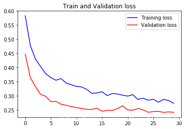
from keras.preprocessing.image import ImageDataGenerator

train_datagen = ImageDataGenerator(
      rescale=1./255,
      rotation_range=40,
      width_shift_range=0.2,
      height_shift_range=0.2,
      shear_range=0.2,
      zoom_range=0.2,
      horizontal_flip=True,
      fill_mode='nearest')

# Note that the validation data should not be augmented!
test_datagen = ImageDataGenerator(rescale=1./255)

train_generator = train_datagen.flow_from_directory(
        # This is the target directory
        train_dir,
        # All images will be resized to 150x150
        target_size=(150, 150),
        batch_size=20,
        # Since we use binary_crossentropy loss, we need binary labels
        class_mode='binary')

validation_generator = test_datagen.flow_from_directory(
        validation_dir,
        target_size=(150, 150),
        batch_size=20,
        class_mode='binary')

model.compile(loss='binary_crossentropy',
              optimizer=optimizers.RMSprop(lr=2e-5),
              metrics=['acc'])

history = model.fit_generator(
      train_generator,
      steps_per_epoch=100,
      epochs=30,
      validation_data=validation_generator,
      validation_steps=50,
      verbose=2)
'''
Found 2000 images belonging to 2 classes.
Found 1000 images belonging to 2 classes.
Epoch 1/30
 - 526s - loss: 0.5844 - acc: 0.6955 - val_loss: 0.4446 - val_acc: 0.8160
Epoch 2/30
 - 520s - loss: 0.4693 - acc: 0.7885 - val_loss: 0.3661 - val_acc: 0.8700
Epoch 3/30
 - 521s - loss: 0.4280 - acc: 0.8055 - val_loss: 0.3229 - val_acc: 0.8710
Epoch 4/30
 - 521s - loss: 0.4052 - acc: 0.8200 - val_loss: 0.2976 - val_acc: 0.8860
Epoch 5/30
 - 520s - loss: 0.3775 - acc: 0.8380 - val_loss: 0.2880 - val_acc: 0.8850
Epoch 6/30
 - 521s - loss: 0.3605 - acc: 0.8430 - val_loss: 0.2758 - val_acc: 0.8930
Epoch 7/30
 - 521s - loss: 0.3538 - acc: 0.8440 - val_loss: 0.2689 - val_acc: 0.8970
Epoch 8/30
 - 521s - loss: 0.3415 - acc: 0.8540 - val_loss: 0.2656 - val_acc: 0.8970
Epoch 9/30
 - 521s - loss: 0.3339 - acc: 0.8575 - val_loss: 0.2678 - val_acc: 0.8980
Epoch 10/30
 - 521s - loss: 0.3229 - acc: 0.8595 - val_loss: 0.2750 - val_acc: 0.8810
Epoch 11/30
 - 521s - loss: 0.3221 - acc: 0.8560 - val_loss: 0.2536 - val_acc: 0.8920
Epoch 12/30
 - 521s - loss: 0.3250 - acc: 0.8600 - val_loss: 0.2635 - val_acc: 0.8870
Epoch 13/30
 - 521s - loss: 0.3263 - acc: 0.8570 - val_loss: 0.2522 - val_acc: 0.8930
Epoch 14/30
 - 521s - loss: 0.3053 - acc: 0.8685 - val_loss: 0.2505 - val_acc: 0.8890
Epoch 15/30
 - 521s - loss: 0.3203 - acc: 0.8665 - val_loss: 0.2459 - val_acc: 0.9020
Epoch 16/30
 - 521s - loss: 0.3107 - acc: 0.8635 - val_loss: 0.2601 - val_acc: 0.8890
Epoch 17/30
 - 521s - loss: 0.2983 - acc: 0.8760 - val_loss: 0.2534 - val_acc: 0.8920
Epoch 18/30
 - 520s - loss: 0.2995 - acc: 0.8780 - val_loss: 0.2457 - val_acc: 0.8970
Epoch 19/30
 - 520s - loss: 0.2951 - acc: 0.8760 - val_loss: 0.2445 - val_acc: 0.8990
Epoch 20/30
 - 521s - loss: 0.2912 - acc: 0.8715 - val_loss: 0.2602 - val_acc: 0.8920
Epoch 21/30
 - 522s - loss: 0.2915 - acc: 0.8760 - val_loss: 0.2375 - val_acc: 0.9070
Epoch 22/30
 - 521s - loss: 0.3073 - acc: 0.8610 - val_loss: 0.2387 - val_acc: 0.9060
Epoch 23/30
 - 521s - loss: 0.2885 - acc: 0.8805 - val_loss: 0.2384 - val_acc: 0.9030
Epoch 24/30
 - 522s - loss: 0.2868 - acc: 0.8770 - val_loss: 0.2403 - val_acc: 0.9030
Epoch 25/30
 - 522s - loss: 0.2883 - acc: 0.8705 - val_loss: 0.2397 - val_acc: 0.9000
Epoch 26/30
 - 521s - loss: 0.2985 - acc: 0.8700 - val_loss: 0.2415 - val_acc: 0.8980
Epoch 27/30
 - 521s - loss: 0.2778 - acc: 0.8775 - val_loss: 0.2552 - val_acc: 0.8960
Epoch 28/30
 - 521s - loss: 0.2842 - acc: 0.8775 - val_loss: 0.2361 - val_acc: 0.9010
Epoch 29/30
 - 522s - loss: 0.2737 - acc: 0.8865 - val_loss: 0.2385 - val_acc: 0.8990
Epoch 30/30
 - 522s - loss: 0.2767 - acc: 0.8745 - val_loss: 0.2423 - val_acc: 0.9000
'''
model.save('cats_and_dogs_small_3.h5')
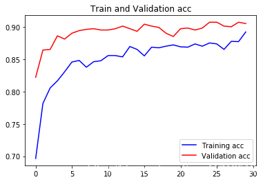
Draw results:
acc = history.history['acc']
val_acc = history.history['val_acc']
loss = history.history['loss']
val_loss = history.history['val_loss']

epochs = range(len(acc))

plt.plot(epochs, acc, 'bo', label='Training acc')
plt.plot(epochs, val_acc, 'b', label='Validation acc')
plt.title('Training and validation accuracy')
plt.legend()

plt.figure()

plt.plot(epochs, loss, 'bo', label='Training loss')
plt.plot(epochs, val_loss, 'b', label='Validation loss')
plt.title('Training and validation loss')
plt.legend()

plt.show()
Fine tuning
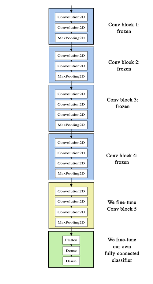
Defrost some layers in the underlying network:
When feature extraction is performed, the user-defined network is added to the trained basic network, the basic network is frozen, and the part added by the training is completed.
Defrost conv_base and freeze individual layers in it.
conv_base.summary()
'''
_________________________________________________________________
Layer (type)                 Output Shape              Param #
=================================================================
input_1 (InputLayer)         (None, 150, 150, 3)       0
_________________________________________________________________
block1_conv1 (Conv2D)        (None, 150, 150, 64)      1792
_________________________________________________________________
block1_conv2 (Conv2D)        (None, 150, 150, 64)      36928
_________________________________________________________________
block1_pool (MaxPooling2D)   (None, 75, 75, 64)        0
_________________________________________________________________
block2_conv1 (Conv2D)        (None, 75, 75, 128)       73856
_________________________________________________________________
block2_conv2 (Conv2D)        (None, 75, 75, 128)       147584
_________________________________________________________________
block2_pool (MaxPooling2D)   (None, 37, 37, 128)       0
_________________________________________________________________
block3_conv1 (Conv2D)        (None, 37, 37, 256)       295168
_________________________________________________________________
block3_conv2 (Conv2D)        (None, 37, 37, 256)       590080
_________________________________________________________________
block3_conv3 (Conv2D)        (None, 37, 37, 256)       590080
_________________________________________________________________
block3_pool (MaxPooling2D)   (None, 18, 18, 256)       0
_________________________________________________________________
block4_conv1 (Conv2D)        (None, 18, 18, 512)       1180160
_________________________________________________________________
block4_conv2 (Conv2D)        (None, 18, 18, 512)       2359808
_________________________________________________________________
block4_conv3 (Conv2D)        (None, 18, 18, 512)       2359808
_________________________________________________________________
block4_pool (MaxPooling2D)   (None, 9, 9, 512)         0
_________________________________________________________________
block5_conv1 (Conv2D)        (None, 9, 9, 512)         2359808
_________________________________________________________________
block5_conv2 (Conv2D)        (None, 9, 9, 512)         2359808
_________________________________________________________________
block5_conv3 (Conv2D)        (None, 9, 9, 512)         2359808
_________________________________________________________________
block5_pool (MaxPooling2D)   (None, 4, 4, 512)         0
=================================================================
Total params: 14,714,688
Trainable params: 14,714,688
Non-trainable params: 0
_________________________________________________________________
'''
The first layer is frozen to the block4_pool layer, while the layers block5_conv1, block5_conv2, and block5_conv3 are updated for training.
conv_base.trainable = True

set_trainable = False
for layer in conv_base.layers:
    if layer.name == 'block5_conv1':
        set_trainable = True
    if set_trainable:
        layer.trainable = True
    else:
        layer.trainable = False
'''
<keras.engine.input_layer.InputLayer object at 0x0000018C750AFA20>
<keras.layers.convolutional.Conv2D object at 0x0000018C750E40F0>
<keras.layers.convolutional.Conv2D object at 0x0000018C7FE9CAC8>
<keras.layers.pooling.MaxPooling2D object at 0x0000018C7FF07FD0>
<keras.layers.convolutional.Conv2D object at 0x0000018C7FEDB5F8>
<keras.layers.convolutional.Conv2D object at 0x0000018C7FF350F0>
<keras.layers.pooling.MaxPooling2D object at 0x0000018C7FF5E470>
<keras.layers.convolutional.Conv2D object at 0x0000018C7FF4C2E8>
<keras.layers.convolutional.Conv2D object at 0x0000018C7FF86E80>
<keras.layers.convolutional.Conv2D object at 0x0000018C7FFB1438>
<keras.layers.pooling.MaxPooling2D object at 0x0000018C7FFC8A90>
<keras.layers.convolutional.Conv2D object at 0x0000018C06008630>
<keras.layers.convolutional.Conv2D object at 0x0000018C060219B0>
<keras.layers.convolutional.Conv2D object at 0x0000018C060490B8>
<keras.layers.pooling.MaxPooling2D object at 0x0000018C0605EC50>
<keras.layers.convolutional.Conv2D object at 0x0000018C060763C8>
<keras.layers.convolutional.Conv2D object at 0x0000018C0609F048>
<keras.layers.convolutional.Conv2D object at 0x0000018C060C5BE0>
<keras.layers.pooling.MaxPooling2D object at 0x0000018C060F2278>
'''
Start fine tuning the network:
The RMSprop optimization function with a low learning rate is used to control the updates to the output of the three-layer network features that we are fine-tuning.
from keras.models import load_model
model = load_model('cats_and_dogs_small_3.h5')
from keras.preprocessing.image import ImageDataGenerator

model.compile(loss='binary_crossentropy',
              optimizer=optimizers.RMSprop(lr=1e-5),
              metrics=['acc'])

history = model.fit_generator(
      train_generator,
      steps_per_epoch=100,
      epochs=100,
      validation_data=validation_generator,
      validation_steps=50)
'''
Epoch 1/100
100/100 [==============================] - 71s 708ms/step - loss: 0.2964 - acc: 0.8740 - val_loss: 0.2679 - val_acc: 0.8940
Epoch 2/100
100/100 [==============================] - 69s 695ms/step - loss: 0.2588 - acc: 0.8950 - val_loss: 0.2117 - val_acc: 0.9130
Epoch 3/100
100/100 [==============================] - 70s 696ms/step - loss: 0.2290 - acc: 0.9045 - val_loss: 0.2136 - val_acc: 0.9130
Epoch 4/100
100/100 [==============================] - 69s 690ms/step - loss: 0.2251 - acc: 0.9090 - val_loss: 0.2173 - val_acc: 0.9130
Epoch 5/100
100/100 [==============================] - 69s 689ms/step - loss: 0.2254 - acc: 0.9075 - val_loss: 0.2012 - val_acc: 0.9180
Epoch 6/100
100/100 [==============================] - 69s 694ms/step - loss: 0.1914 - acc: 0.9230 - val_loss: 0.1999 - val_acc: 0.9270
Epoch 7/100
100/100 [==============================] - 69s 694ms/step - loss: 0.1788 - acc: 0.9320 - val_loss: 0.2214 - val_acc: 0.9180
Epoch 8/100
100/100 [==============================] - 69s 689ms/step - loss: 0.1718 - acc: 0.9275 - val_loss: 0.2047 - val_acc: 0.9210
Epoch 9/100
100/100 [==============================] - 69s 688ms/step - loss: 0.1522 - acc: 0.9340 - val_loss: 0.2339 - val_acc: 0.9120
Epoch 10/100
100/100 [==============================] - 69s 692ms/step - loss: 0.1413 - acc: 0.9440 - val_loss: 0.1962 - val_acc: 0.9260
Epoch 11/100
100/100 [==============================] - 69s 688ms/step - loss: 0.1683 - acc: 0.9330 - val_loss: 0.2370 - val_acc: 0.9080
Epoch 12/100
100/100 [==============================] - 69s 694ms/step - loss: 0.1428 - acc: 0.9415 - val_loss: 0.1867 - val_acc: 0.9290
Epoch 13/100
100/100 [==============================] - 69s 687ms/step - loss: 0.1289 - acc: 0.9540 - val_loss: 0.1870 - val_acc: 0.9310
Epoch 14/100
100/100 [==============================] - 69s 689ms/step - loss: 0.1386 - acc: 0.9440 - val_loss: 0.1763 - val_acc: 0.9290
Epoch 15/100
100/100 [==============================] - 69s 695ms/step - loss: 0.1281 - acc: 0.9475 - val_loss: 0.1794 - val_acc: 0.9300
Epoch 16/100
100/100 [==============================] - 69s 694ms/step - loss: 0.1126 - acc: 0.9545 - val_loss: 0.1843 - val_acc: 0.9340
Epoch 17/100
100/100 [==============================] - 69s 690ms/step - loss: 0.0951 - acc: 0.9595 - val_loss: 0.1679 - val_acc: 0.9310
Epoch 18/100
100/100 [==============================] - 69s 688ms/step - loss: 0.1109 - acc: 0.9565 - val_loss: 0.1779 - val_acc: 0.9340
Epoch 19/100
100/100 [==============================] - 69s 691ms/step - loss: 0.0944 - acc: 0.9670 - val_loss: 0.1766 - val_acc: 0.9320
Epoch 20/100
100/100 [==============================] - 69s 689ms/step - loss: 0.0942 - acc: 0.9670 - val_loss: 0.2022 - val_acc: 0.9250
Epoch 21/100
100/100 [==============================] - 69s 690ms/step - loss: 0.0921 - acc: 0.9635 - val_loss: 0.2021 - val_acc: 0.9260
Epoch 22/100
100/100 [==============================] - 69s 691ms/step - loss: 0.0825 - acc: 0.9670 - val_loss: 0.1876 - val_acc: 0.9320
Epoch 23/100
100/100 [==============================] - 69s 689ms/step - loss: 0.1010 - acc: 0.9630 - val_loss: 0.1837 - val_acc: 0.9360
Epoch 24/100
100/100 [==============================] - 69s 691ms/step - loss: 0.0847 - acc: 0.9670 - val_loss: 0.1988 - val_acc: 0.9350
Epoch 25/100
100/100 [==============================] - 69s 690ms/step - loss: 0.0731 - acc: 0.9705 - val_loss: 0.2018 - val_acc: 0.9350
Epoch 26/100
100/100 [==============================] - 69s 689ms/step - loss: 0.0827 - acc: 0.9695 - val_loss: 0.1748 - val_acc: 0.9400
Epoch 27/100
100/100 [==============================] - 69s 689ms/step - loss: 0.0722 - acc: 0.9755 - val_loss: 0.2203 - val_acc: 0.9330
Epoch 28/100
100/100 [==============================] - 69s 689ms/step - loss: 0.0680 - acc: 0.9735 - val_loss: 0.2063 - val_acc: 0.9280
Epoch 29/100
100/100 [==============================] - 69s 689ms/step - loss: 0.0654 - acc: 0.9710 - val_loss: 0.1923 - val_acc: 0.9360
Epoch 30/100
100/100 [==============================] - 69s 694ms/step - loss: 0.0733 - acc: 0.9710 - val_loss: 0.1965 - val_acc: 0.9320
Epoch 31/100
100/100 [==============================] - 69s 692ms/step - loss: 0.0708 - acc: 0.9760 - val_loss: 0.2125 - val_acc: 0.9290
Epoch 32/100
100/100 [==============================] - 69s 689ms/step - loss: 0.0669 - acc: 0.9745 - val_loss: 0.2035 - val_acc: 0.9350
Epoch 33/100
100/100 [==============================] - 69s 690ms/step - loss: 0.0679 - acc: 0.9735 - val_loss: 0.2199 - val_acc: 0.9270
Epoch 34/100
100/100 [==============================] - 69s 692ms/step - loss: 0.0628 - acc: 0.9785 - val_loss: 0.1928 - val_acc: 0.9310
Epoch 35/100
100/100 [==============================] - 69s 687ms/step - loss: 0.0664 - acc: 0.9770 - val_loss: 0.2173 - val_acc: 0.9290
Epoch 36/100
100/100 [==============================] - 69s 691ms/step - loss: 0.0515 - acc: 0.9820 - val_loss: 0.2261 - val_acc: 0.9340
Epoch 37/100
100/100 [==============================] - 69s 692ms/step - loss: 0.0555 - acc: 0.9785 - val_loss: 0.3316 - val_acc: 0.9160
Epoch 38/100
100/100 [==============================] - 69s 688ms/step - loss: 0.0558 - acc: 0.9790 - val_loss: 0.2359 - val_acc: 0.9340
Epoch 39/100
100/100 [==============================] - 69s 692ms/step - loss: 0.0400 - acc: 0.9875 - val_loss: 0.2345 - val_acc: 0.9350
Epoch 40/100
100/100 [==============================] - 69s 695ms/step - loss: 0.0504 - acc: 0.9830 - val_loss: 0.2222 - val_acc: 0.9370
Epoch 41/100
100/100 [==============================] - 69s 687ms/step - loss: 0.0437 - acc: 0.9835 - val_loss: 0.2325 - val_acc: 0.9390
Epoch 42/100
100/100 [==============================] - 69s 688ms/step - loss: 0.0455 - acc: 0.9830 - val_loss: 0.2271 - val_acc: 0.9410
Epoch 43/100
100/100 [==============================] - 69s 688ms/step - loss: 0.0557 - acc: 0.9805 - val_loss: 0.2746 - val_acc: 0.9300
Epoch 44/100
100/100 [==============================] - 69s 694ms/step - loss: 0.0450 - acc: 0.9840 - val_loss: 0.3066 - val_acc: 0.9230
Epoch 45/100
100/100 [==============================] - 69s 687ms/step - loss: 0.0536 - acc: 0.9810 - val_loss: 0.2126 - val_acc: 0.9330
Epoch 46/100
100/100 [==============================] - 69s 689ms/step - loss: 0.0477 - acc: 0.9810 - val_loss: 0.1954 - val_acc: 0.9400
Epoch 47/100
100/100 [==============================] - 69s 687ms/step - loss: 0.0360 - acc: 0.9885 - val_loss: 0.2033 - val_acc: 0.9410
Epoch 48/100
100/100 [==============================] - 69s 687ms/step - loss: 0.0405 - acc: 0.9820 - val_loss: 0.2188 - val_acc: 0.9330
Epoch 49/100
100/100 [==============================] - 68s 685ms/step - loss: 0.0318 - acc: 0.9880 - val_loss: 0.2992 - val_acc: 0.9240
Epoch 50/100
100/100 [==============================] - 69s 690ms/step - loss: 0.0308 - acc: 0.9900 - val_loss: 0.2760 - val_acc: 0.9280
Epoch 51/100
100/100 [==============================] - 69s 688ms/step - loss: 0.0429 - acc: 0.9855 - val_loss: 0.2365 - val_acc: 0.9360
Epoch 52/100
100/100 [==============================] - 69s 687ms/step - loss: 0.0435 - acc: 0.9845 - val_loss: 0.2321 - val_acc: 0.9400
Epoch 53/100
100/100 [==============================] - 69s 686ms/step - loss: 0.0306 - acc: 0.9895 - val_loss: 0.2982 - val_acc: 0.9260
Epoch 54/100
100/100 [==============================] - 69s 686ms/step - loss: 0.0406 - acc: 0.9850 - val_loss: 0.3509 - val_acc: 0.9260
Epoch 55/100
100/100 [==============================] - 69s 691ms/step - loss: 0.0374 - acc: 0.9890 - val_loss: 0.2440 - val_acc: 0.9350
Epoch 56/100
100/100 [==============================] - 69s 690ms/step - loss: 0.0313 - acc: 0.9880 - val_loss: 0.2671 - val_acc: 0.9300
Epoch 57/100
100/100 [==============================] - 69s 688ms/step - loss: 0.0264 - acc: 0.9865 - val_loss: 0.2277 - val_acc: 0.9340
Epoch 58/100
100/100 [==============================] - 69s 685ms/step - loss: 0.0286 - acc: 0.9890 - val_loss: 0.3027 - val_acc: 0.9310
Epoch 59/100
100/100 [==============================] - 69s 691ms/step - loss: 0.0332 - acc: 0.9865 - val_loss: 0.2370 - val_acc: 0.9330
Epoch 60/100
100/100 [==============================] - 69s 687ms/step - loss: 0.0251 - acc: 0.9900 - val_loss: 0.2270 - val_acc: 0.9400
Epoch 61/100
100/100 [==============================] - 69s 689ms/step - loss: 0.0345 - acc: 0.9880 - val_loss: 0.3246 - val_acc: 0.9190
Epoch 62/100
100/100 [==============================] - 69s 691ms/step - loss: 0.0360 - acc: 0.9905 - val_loss: 0.3061 - val_acc: 0.9290
Epoch 63/100
100/100 [==============================] - 69s 685ms/step - loss: 0.0405 - acc: 0.9855 - val_loss: 0.2458 - val_acc: 0.9390
Epoch 64/100
100/100 [==============================] - 69s 686ms/step - loss: 0.0241 - acc: 0.9905 - val_loss: 0.2371 - val_acc: 0.9350
Epoch 65/100
100/100 [==============================] - 68s 685ms/step - loss: 0.0223 - acc: 0.9920 - val_loss: 0.2663 - val_acc: 0.9420
Epoch 66/100
100/100 [==============================] - 69s 688ms/step - loss: 0.0325 - acc: 0.9900 - val_loss: 0.2829 - val_acc: 0.9340
Epoch 67/100
100/100 [==============================] - 69s 688ms/step - loss: 0.0319 - acc: 0.9855 - val_loss: 0.2462 - val_acc: 0.9410
Epoch 68/100
100/100 [==============================] - 68s 684ms/step - loss: 0.0314 - acc: 0.9900 - val_loss: 0.2452 - val_acc: 0.9400
Epoch 69/100
100/100 [==============================] - 69s 689ms/step - loss: 0.0217 - acc: 0.9920 - val_loss: 0.2276 - val_acc: 0.9400
Epoch 70/100
100/100 [==============================] - 69s 691ms/step - loss: 0.0316 - acc: 0.9895 - val_loss: 0.3000 - val_acc: 0.9320
Epoch 71/100
100/100 [==============================] - 69s 685ms/step - loss: 0.0235 - acc: 0.9900 - val_loss: 0.2419 - val_acc: 0.9380
Epoch 72/100
100/100 [==============================] - 68s 684ms/step - loss: 0.0254 - acc: 0.9890 - val_loss: 0.2744 - val_acc: 0.9270
Epoch 73/100
100/100 [==============================] - 69s 688ms/step - loss: 0.0213 - acc: 0.9935 - val_loss: 0.2577 - val_acc: 0.9360
Epoch 74/100
100/100 [==============================] - 69s 687ms/step - loss: 0.0234 - acc: 0.9900 - val_loss: 0.5941 - val_acc: 0.8910
Epoch 75/100
100/100 [==============================] - 69s 686ms/step - loss: 0.0229 - acc: 0.9910 - val_loss: 0.2376 - val_acc: 0.9410
Epoch 76/100
100/100 [==============================] - 68s 684ms/step - loss: 0.0269 - acc: 0.9895 - val_loss: 0.2192 - val_acc: 0.9400
Epoch 77/100
100/100 [==============================] - 69s 690ms/step - loss: 0.0306 - acc: 0.9895 - val_loss: 0.4235 - val_acc: 0.9180
Epoch 78/100
100/100 [==============================] - 69s 688ms/step - loss: 0.0297 - acc: 0.9870 - val_loss: 0.4058 - val_acc: 0.9150
Epoch 79/100
100/100 [==============================] - 68s 685ms/step - loss: 0.0185 - acc: 0.9920 - val_loss: 0.2406 - val_acc: 0.9350
Epoch 80/100
100/100 [==============================] - 68s 682ms/step - loss: 0.0231 - acc: 0.9925 - val_loss: 0.2911 - val_acc: 0.9350
Epoch 81/100
100/100 [==============================] - 68s 685ms/step - loss: 0.0210 - acc: 0.9925 - val_loss: 0.2490 - val_acc: 0.9390
Epoch 82/100
100/100 [==============================] - 68s 683ms/step - loss: 0.0285 - acc: 0.9900 - val_loss: 0.2651 - val_acc: 0.9400
Epoch 83/100
100/100 [==============================] - 69s 686ms/step - loss: 0.0238 - acc: 0.9915 - val_loss: 0.2630 - val_acc: 0.9420
Epoch 84/100
100/100 [==============================] - 69s 691ms/step - loss: 0.0139 - acc: 0.9945 - val_loss: 0.4327 - val_acc: 0.9170
Epoch 85/100
100/100 [==============================] - 70s 696ms/step - loss: 0.0318 - acc: 0.9885 - val_loss: 0.3970 - val_acc: 0.9170
Epoch 86/100
100/100 [==============================] - 69s 689ms/step - loss: 0.0212 - acc: 0.9920 - val_loss: 0.2888 - val_acc: 0.9360
Epoch 87/100
100/100 [==============================] - 69s 691ms/step - loss: 0.0271 - acc: 0.9900 - val_loss: 0.3411 - val_acc: 0.9280
Epoch 88/100
100/100 [==============================] - 69s 689ms/step - loss: 0.0168 - acc: 0.9955 - val_loss: 0.2189 - val_acc: 0.9480
Epoch 89/100
100/100 [==============================] - 70s 697ms/step - loss: 0.0233 - acc: 0.9920 - val_loss: 0.2459 - val_acc: 0.9410
Epoch 90/100
100/100 [==============================] - 69s 690ms/step - loss: 0.0224 - acc: 0.9915 - val_loss: 0.2352 - val_acc: 0.9400
Epoch 91/100
100/100 [==============================] - 70s 699ms/step - loss: 0.0189 - acc: 0.9925 - val_loss: 0.2632 - val_acc: 0.9380
Epoch 92/100
100/100 [==============================] - 69s 694ms/step - loss: 0.0163 - acc: 0.9940 - val_loss: 0.3046 - val_acc: 0.9360
Epoch 93/100
100/100 [==============================] - 69s 695ms/step - loss: 0.0099 - acc: 0.9980 - val_loss: 0.3264 - val_acc: 0.9350
Epoch 94/100
100/100 [==============================] - 69s 694ms/step - loss: 0.0174 - acc: 0.9950 - val_loss: 0.2712 - val_acc: 0.9370
Epoch 95/100
100/100 [==============================] - 69s 691ms/step - loss: 0.0132 - acc: 0.9965 - val_loss: 0.3202 - val_acc: 0.9330
Epoch 96/100
100/100 [==============================] - 69s 695ms/step - loss: 0.0126 - acc: 0.9945 - val_loss: 0.2944 - val_acc: 0.9330
Epoch 97/100
100/100 [==============================] - 70s 695ms/step - loss: 0.0236 - acc: 0.9940 - val_loss: 0.3391 - val_acc: 0.9340
Epoch 98/100
100/100 [==============================] - 69s 689ms/step - loss: 0.0241 - acc: 0.9910 - val_loss: 0.2671 - val_acc: 0.9360
Epoch 99/100
100/100 [==============================] - 69s 695ms/step - loss: 0.0231 - acc: 0.9915 - val_loss: 0.2538 - val_acc: 0.9400
Epoch 100/100
100/100 [==============================] - 69s 693ms/step - loss: 0.0219 - acc: 0.9935 - val_loss: 0.2560 - val_acc: 0.9370
'''
model.save('cats_and_dogs_small_4.h5')
Draw results:
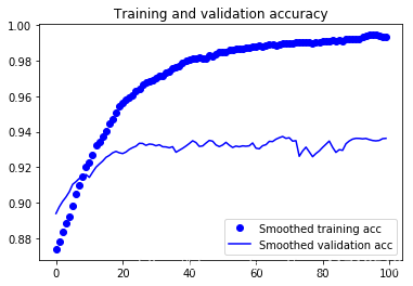
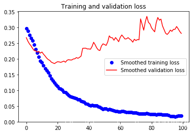
acc = history.history['acc']
val_acc = history.history['val_acc']
loss = history.history['loss']
val_loss = history.history['val_loss']

epochs = range(len(acc))

plt.plot(epochs, acc, 'bo', label='Training acc')
plt.plot(epochs, val_acc, 'b', label='Validation acc')
plt.title('Training and validation accuracy')
plt.legend()

plt.figure()

plt.plot(epochs, loss, 'bo', label='Training loss')
plt.plot(epochs, val_loss, 'b', label='Validation loss')
plt.title('Training and validation loss')
plt.legend()

plt.show()
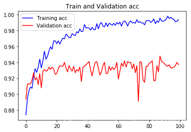
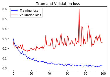
These curves look very noisy, and to make them more readable, we can smooth them by calculating the exponential moving average instead of each loss and accuracy.
def smooth_curve(points, factor=0.8):
  smoothed_points = []
  for point in points:
    if smoothed_points:
      previous = smoothed_points[-1]
      smoothed_points.append(previous * factor + point * (1 - factor))
    else:
      smoothed_points.append(point)
  return smoothed_points

plt.plot(epochs,
         smooth_curve(acc), 'bo', label='Smoothed training acc')
plt.plot(epochs,
         smooth_curve(val_acc), 'b', label='Smoothed validation acc')
plt.title('Training and validation accuracy')
plt.legend()

plt.figure()

plt.plot(epochs,
         smooth_curve(loss), 'bo', label='Smoothed training loss')
plt.plot(epochs,
         smooth_curve(val_loss), 'b', label='Smoothed validation loss')
plt.title('Training and validation loss')
plt.legend()

plt.show()
Evaluation model:
test_generator = test_datagen.flow_from_directory(
        test_dir,
        target_size=(150, 150),
        batch_size=20,
        class_mode='binary')

test_loss, test_acc = model.evaluate_generator(test_generator, steps=50)
print('test acc:', test_acc)
'''
Found 1000 images belonging to 2 classes.
test acc: 0.9730000052452088
'''
Summary
1.convnet is the best machine learning model for computer vision tasks.Even on a very small dataset, you can start training from scratch and get impressive results.
2. Overfitting will be the main problem on small datasets.Data expansion is a powerful way to combat over-fitting when processing image data.
3. Feature extraction makes it easy to use an existing convnet on a new dataset.This is also a very valuable technique for processing small image data sets.
4. As a supplement to feature extraction, fine-tuning can also be used to apply some of the features learned from existing models to new problems, which can further improve performance.

