Counter Plot, Contour Demo, Creating a "meshgrid", Calculation of the Values, etc

Posted by dunn_cann on Tue, 08 Mar 2022 22:48:36 +0100

21. Contour map (Counter Plot)
21.1.Contour Demo
21.2.Creating a "meshgrid"
21.3.Calculation of the Values
21.4.Changing the Colours and the Line Style
21.5.Filled Contours
21.6.Individual Colours

21. Contour map (Counter Plot)

The contour line (or contour line) of two variable functions is a curve with constant value. It is the cross-section of the three-dimensional graph of the function f(x,y) parallel to the X, y plane.

For example, climbing lines are used in geography and meteorology. In cartography, contour lines connect points of equal height above a given level, such as mean sea level.

We can also more generally say that the isoline of a function with two variables is a curve connecting points with the same value.

Contour and contour both draw three-dimensional contour maps. The difference is that contour() draws contour lines and contour() fills the contour.

21.1.Contour Demo

Give an example of a simple isoline drawing: isolines on an image, as well as color bars for isolines and marked contours.

import matplotlib
import numpy as np
import matplotlib.cm as cm
import matplotlib.pyplot as plt


delta = 0.025
x = np.arange(-3.0, 3.0, delta)
y = np.arange(-2.0, 2.0, delta)
X, Y = np.meshgrid(x, y)
Z1 = np.exp(-X**2 - Y**2)
Z2 = np.exp(-(X - 1)**2 - (Y - 1)**2)
Z = (Z1 - Z2) * 2

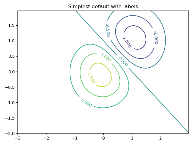
Create a simple contour map with labels using the default colors. The inline parameter of clabel controls whether labels are drawn on the segments of isolines, thereby removing the lines below the labels.

fig, ax = plt.subplots()
CS = ax.contour(X, Y, Z)
ax.clabel(CS, inline=1, fontsize=10)
ax.set_title('Simplest default with labels')

Namely:

import matplotlib
import numpy as np
import matplotlib.cm as cm
import matplotlib.pyplot as plt


delta = 0.025
x = np.arange(-3.0, 3.0, delta)
y = np.arange(-2.0, 2.0, delta)
X, Y = np.meshgrid(x, y)
Z1 = np.exp(-X**2 - Y**2)
Z2 = np.exp(-(X - 1)**2 - (Y - 1)**2)
Z = (Z1 - Z2) * 2

fig, ax = plt.subplots()
CS = ax.contour(X, Y, Z)
ax.clabel(CS, inline=1, fontsize=10)
ax.set_title('Simplest default with labels')

plt.show()

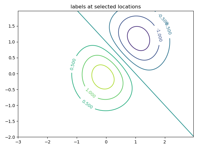
You can manually place isoline labels through the list of locations in the provided data coordinates.

fig, ax = plt.subplots()
CS = ax.contour(X, Y, Z)
manual_locations = [(-1, -1.4), (-0.62, -0.7), (-2, 0.5), (1.7, 1.2), (2.0, 1.4), (2.4, 1.7)]
ax.clabel(CS, inline=1, fontsize=10, manual=manual_locations)
ax.set_title('labels at selected locations')

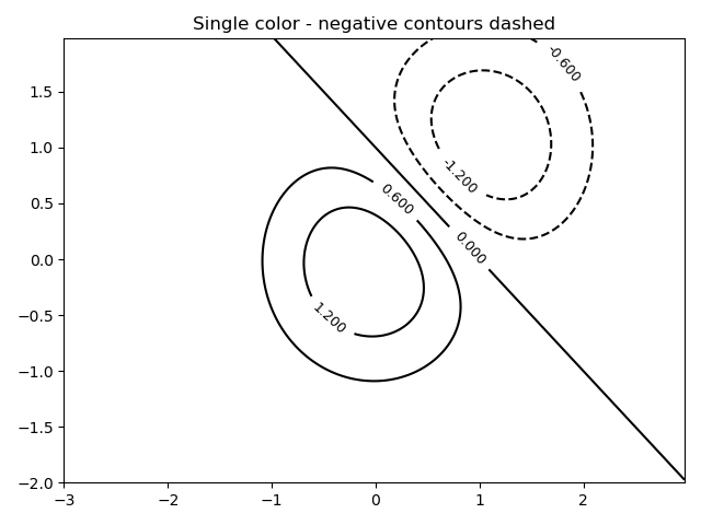
You can force all isolines to be the same color.

import matplotlib
import numpy as np
import matplotlib.cm as cm
import matplotlib.pyplot as plt

delta = 0.025
x = np.arange(-3.0, 3.0, delta)
y = np.arange(-2.0, 2.0, delta)
X, Y = np.meshgrid(x, y)
Z1 = np.exp(-X**2 - Y**2)
Z2 = np.exp(-(X - 1)**2 - (Y - 1)**2)
Z = (Z1 - Z2) * 2

fig, ax = plt.subplots()
CS = ax.contour(X, Y, Z, 6,
                colors='k'    # negative contours will be dashed by default
                )
ax.clabel(CS, fontsize=9, inline=1)
ax.set_title('Single color - negative contours dashed')

plt.show()

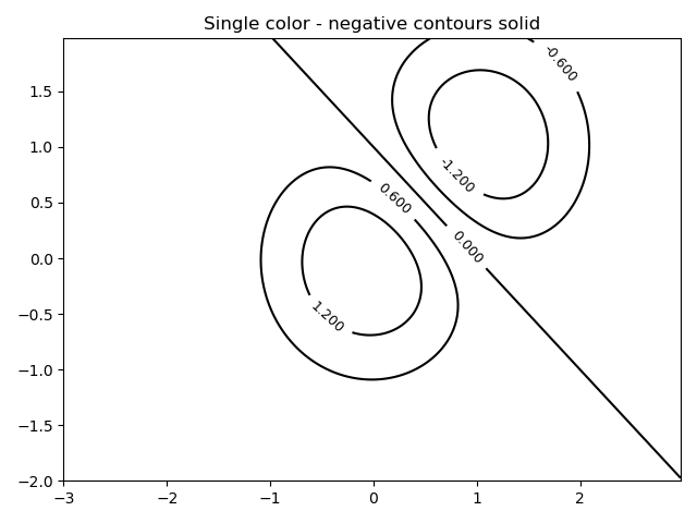
You can set a negative isoline to a solid line instead of a dashed line:

import matplotlib
import numpy as np
import matplotlib.cm as cm
import matplotlib.pyplot as plt


delta = 0.025
x = np.arange(-3.0, 3.0, delta)
y = np.arange(-2.0, 2.0, delta)
X, Y = np.meshgrid(x, y)
Z1 = np.exp(-X**2 - Y**2)
Z2 = np.exp(-(X - 1)**2 - (Y - 1)**2)
Z = (Z1 - Z2) * 2

matplotlib.rcParams['contour.negative_linestyle'] = 'solid'
fig, ax = plt.subplots()
CS = ax.contour(X, Y, Z, 6,
                 colors='k',  # negative contours will be dashed by default
                 )
ax.clabel(CS, fontsize=9, inline=1)
ax.set_title('Single color - negative contours solid')

plt.show()

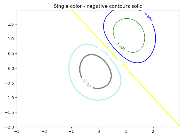
You can manually specify the color of the isoline:

import matplotlib
import numpy as np
import matplotlib.cm as cm
import matplotlib.pyplot as plt

delta = 0.025
x = np.arange(-3.0, 3.0, delta)
y = np.arange(-2.0, 2.0, delta)
X, Y = np.meshgrid(x, y)
Z1 = np.exp(-X**2 - Y**2)
Z2 = np.exp(-(X - 1)**2 - (Y - 1)**2)
Z = (Z1 - Z2) * 2

matplotlib.rcParams['contour.negative_linestyle'] = 'solid'
fig, ax = plt.subplots()
CS = ax.contour(X, Y, Z, 6,
                linewidths=np.arange(.5, 4, .5),
                 colors=('r', 'green', 'blue', (1, 1, 0), '#afeeee', '0.5'),  # negative contours will be dashed by default
                 )
ax.clabel(CS, fontsize=9, inline=1)
ax.set_title('Single color - negative contours solid')

plt.show()

You can use a color map to specify colors. The default color map will be used for isolines.

import matplotlib
import numpy as np
import matplotlib.cm as cm
import matplotlib.pyplot as plt

delta = 0.025
x = np.arange(-3.0, 3.0, delta)
y = np.arange(-2.0, 2.0, delta)
X, Y = np.meshgrid(x, y)
Z1 = np.exp(-X**2 - Y**2)
Z2 = np.exp(-(X - 1)**2 - (Y - 1)**2)
Z = (Z1 - Z2) * 2

fig, ax = plt.subplots()
im = ax.imshow(Z, interpolation='bilinear', origin='lower',
                cmap=cm.gray, extent=(-3, 3, -2, 2))
levels = np.arange(-1.2, 1.6, 0.2)
CS = ax.contour(Z, levels, origin='lower', cmap='flag',
                linewidths=2, extent=(-3, 3, -2, 2))

# Thicken the zero contour.
zc = CS.collections[6]
plt.setp(zc, linewidth=4)

ax.clabel(CS, levels[1::2],  # label every second level
          inline=1, fmt='%1.1f', fontsize=14)

# make a colorbar for the contour lines
CB = fig.colorbar(CS, shrink=0.8, extend='both')

ax.set_title('Lines with colorbar')

# We can still add a colorbar for the image, too.
CBI = fig.colorbar(im, orientation='horizontal', shrink=0.8)

# This makes the original colorbar look a bit out of place,
# so let's improve its position.

l, b, w, h = ax.get_position().bounds
ll, bb, ww, hh = CB.ax.get_position().bounds
CB.ax.set_position([ll, b + 0.1*h, ww, h*0.8])


plt.show()

21.2.Creating a "meshgrid"

import numpy as np

xlist = np.linspace(-3.0, 3.0, 3)
ylist = np.linspace(-3.0, 3.0, 4)
X, Y = np.meshgrid(xlist, ylist)
print(xlist)
print(ylist)
print(X)
print(Y)
"""
Output result:
[-3.  0.  3.]
[-3. -1.  1.  3.]
[[-3.  0.  3.]
 [-3.  0.  3.]
 [-3.  0.  3.]
 [-3.  0.  3.]]
[[-3. -3. -3.]
 [-1. -1. -1.]
 [ 1.  1.  1.]
 [ 3.  3.  3.]]
"""

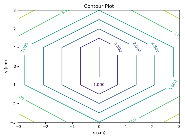
21.3.Calculation of the Values

import numpy as np
import matplotlib.pyplot as plt

xlist = np.linspace(-3.0, 3.0, 3)
ylist = np.linspace(-3.0, 3.0, 4)
X, Y = np.meshgrid(xlist, ylist)
Z = np.sqrt(X**2 + Y**2)
print(Z)
"""
Output result:
[[4.24264069 3.         4.24264069]
 [3.16227766 1.         3.16227766]
 [3.16227766 1.         3.16227766]
 [4.24264069 3.         4.24264069]]
"""

plt.figure()
cp = plt.contour(X, Y, Z)
plt.clabel(cp, inline=True,
          fontsize=10)
plt.title('Contour Plot')
plt.xlabel('x (cm)')
plt.ylabel('y (cm)')
plt.show()

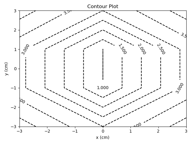
21.4.Changing the Colours and the Line Style

import numpy as np
import matplotlib.pyplot as plt

xlist = np.linspace(-3.0, 3.0, 3)
ylist = np.linspace(-3.0, 3.0, 4)
X, Y = np.meshgrid(xlist, ylist)
Z = np.sqrt(X**2 + Y**2)
print(Z)
"""
Output result:
[[4.24264069 3.         4.24264069]
 [3.16227766 1.         3.16227766]
 [3.16227766 1.         3.16227766]
 [4.24264069 3.         4.24264069]]
"""

plt.figure()
cp = plt.contour(X, Y, Z, colors='black', linestyles='dashed')
plt.clabel(cp, inline=True,
          fontsize=10)
plt.title('Contour Plot')
plt.xlabel('x (cm)')
plt.ylabel('y (cm)')
plt.show()

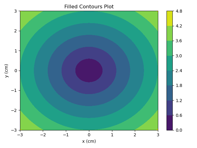
21.5.Filled Contours

import numpy as np
import matplotlib.pyplot as plt
xlist = np.linspace(-3.0, 3.0, 100)
ylist = np.linspace(-3.0, 3.0, 100)
X, Y = np.meshgrid(xlist, ylist)
Z = np.sqrt(X**2 + Y**2)
plt.figure()
cp = plt.contourf(X, Y, Z)
plt.colorbar(cp)
plt.title('Filled Contours Plot')
plt.xlabel('x (cm)')
plt.ylabel('y (cm)')
plt.show()

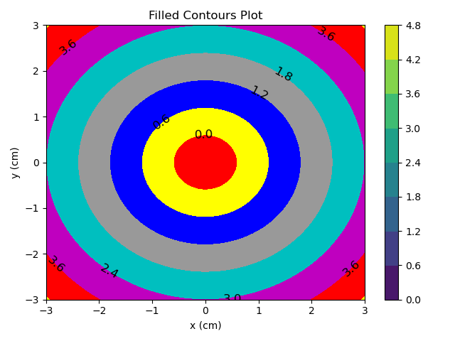
21.6.Individual Colours

import numpy as np
import matplotlib.pyplot as plt
xlist = np.linspace(-3.0, 3.0, 100)
ylist = np.linspace(-3.0, 3.0, 100)
X, Y = np.meshgrid(xlist, ylist)
Z = np.sqrt(X**2 + Y**2)
plt.figure()
contour = plt.contourf(X, Y, Z)
plt.clabel(contour, colors = 'k', fmt = '%2.1f', fontsize=12)
c = ('#ff0000', '#ffff00', '#0000FF', '0.6', 'c', 'm')
contour_filled = plt.contourf(X, Y, Z, colors=c)
plt.colorbar(contour)
plt.title('Filled Contours Plot')
plt.xlabel('x (cm)')
plt.ylabel('y (cm)')
plt.show()

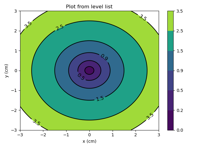
21.7.Levels

So far, levels are determined automatically by contour and contour. You can define them manually by providing a list of levels as the fourth parameter. If you use isolines, isolines are drawn for each value in the list. For contour, a colored area is filled between the values in the list.

import numpy as np
import matplotlib.pyplot as plt
xlist = np.linspace(-3.0, 3.0, 100)
ylist = np.linspace(-3.0, 3.0, 100)
X, Y = np.meshgrid(xlist, ylist)
Z = np.sqrt(X ** 2 + Y ** 2 )
plt.figure()
levels = [0.0, 0.2, 0.5, 0.9, 1.5, 2.5, 3.5]
contour = plt.contour(X, Y, Z, levels, colors='k')
plt.clabel(contour, colors = 'k', fmt = '%2.1f', fontsize=12)
contour_filled = plt.contourf(X, Y, Z, levels)
plt.colorbar(contour_filled)
plt.title('Plot from level list')
plt.xlabel('x (cm)')
plt.ylabel('y (cm)')
plt.show()

Programmer Think