Take Alipay's Sesame credit as an example, its value range is 350-950 points. It is generally believed that the higher the score, the better the credit and the lower the default rate of personal business. Here is also a personal credit scoring tool similar to FICO scoring.

The idea of FICO scoring is: collect / analyze / convert a large number of user data with multiple attributes, use various statistical indicators (such as correlation coefficient / chi square check / variance expansion coefficient, etc.) to choose / copy / combine attributes, and finally get a quantitative / comprehensive / comparable score. On the one hand, the score reflects the quality of the user's historical credit record, on the other hand, it implies the possibility of default in the future.

The original data used here mainly includes the customer's personal information (including gender / age / job / marital status / educational status, etc.) / account information (including the number of various accounts / deposit and loan balance, etc.), as well as the classification label of whether the customer has defaulted.

After the data set is processed, it needs to go through the process of data box / attribute selection and the conversion between discrete classification labels and continuous credit scoring results.

I Import data

#Import package
import pandas as pd
import numpy as np
import matplotlib.pyplot as plt

#View raw data
data = pd.read_csv('credit.csv')
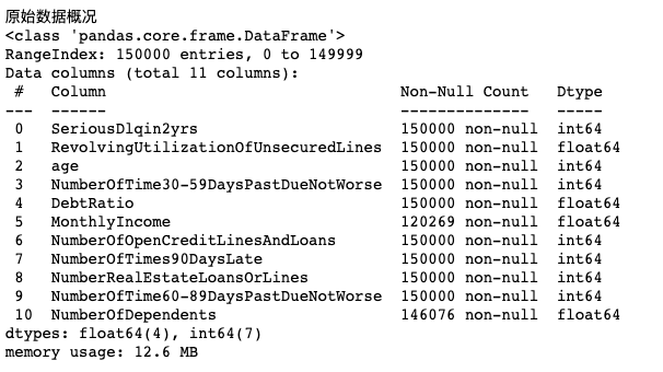
print('Raw data overview')
data.info()
#The data is 12.6m and there are 11 attributes. There are two attributes, MonthlyIncome and NumberOfDependents, which have null values

The data is 12.6M and has 11 attributes. There are two attributes, MonthlyIncome and NumberOfDependents, which have null values

II Data cleaning
Because there are missing values in MonthlyIncome and NumberOfDependents, they need to be processed. The common method is 1 Fill in the blank with upper and lower values; 2. Fill in the blank with the attribute mean value. But each has its own shortcomings. A set is defined here_ Missing function is used to fill in the random forest regression algorithm to fill in the missing values.

#Data cleaning
#The random forest method is used to predict and fill the missing value of MonthlyIncome. Set is defined here_ Missing function
from sklearn.ensemble import RandomForestRegressor
def set_missing(df):
    print('Random forest regression fill 0 value:')
    process_df = df.iloc[:,[5,0,1,2,3,4,6,7,8,9]]
    #Advance the monthly income in column 5 to column 0 as a label to facilitate subsequent data division
    #They were divided into two groups with missing values
    known = process_df.loc[process_df['MonthlyIncome']!=0].values
    unknown = process_df.loc[process_df['MonthlyIncome']==0].values
    X = known[:,1:]
    y = known[:,0]
    #Training random forest regression algorithm with x,y
    rfr = RandomForestRegressor(random_state=0,n_estimators=200,max_depth=3,n_jobs=-1)
    rfr.fit(X,y)
    #The obtained model is used for missing value prediction
    predicted = rfr.predict(unknown[:,1:]).round(0)
    #The obtained prediction results fill the original missing data
    df.loc[df['MonthlyIncome'] == 0,'MonthlyIncome'] = predicted
    return df

Define outlier_ It is used to delete the outlier in the processing function
The method used here is data box Division: divide the value of the attribute into several segments (box), and replace the data falling within the same box with a unified value.

#Delete the outliers in the attribute, find out the outliers, and first calculate the maximum and minimum thresholds as the deletion criteria
#Minimum threshold = first quartile - 1.5 * (third quartile - first quartile)
#Maximum threshold = third quartile + 1.5 * (third quartile - first quartile)
#   Rows with < minimum threshold and > maximum threshold are deleted
#Outlier defined_ The processing function is used to process outlier data points

def outlier_processing(df,cname):
    s = df[cname]
    onequater = s.quantile(0.25)
    threequater = s.quantile(0.75)
    irq = threequater - onequater
    min = onequater - 1.5*irq
    max = threequater + 1.5*irq
    df = df[df[cname]<=max]
    df = df[df[cname]>=min]
    return df

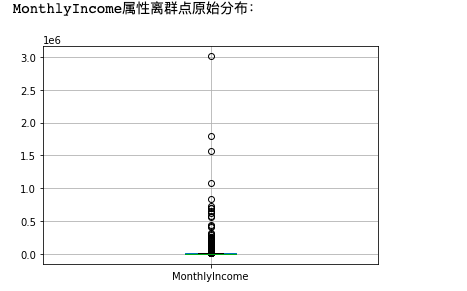
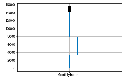
MonthlyIncome original distribution map and processed distribution map

#Data collation of MonthlyIncome column
print('MonthlyIncome Original distribution of attribute outliers:')
data[['MonthlyIncome']].boxplot()
plt.savefig('MonthlyIncome1.png',dpi = 300,bbox_inches = 'tight')
plt.show()
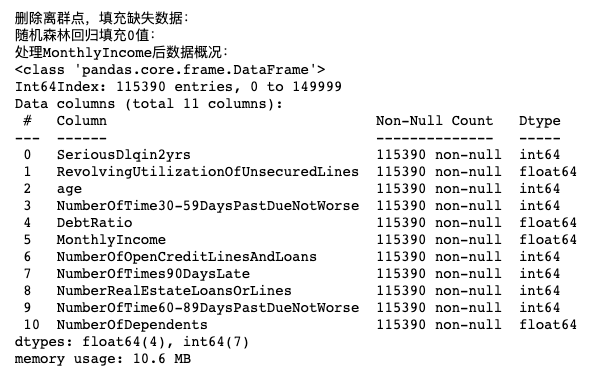
print('Delete outliers and fill in missing data:')
data = outlier_processing(data, 'MonthlyIncome')#Delete outliers
data = set_missing(data)#Fill in missing data
print('handle MonthlyIncome Post data overview:')
data.info()#View collated data
#image display
data[['MonthlyIncome']].boxplot()#Box diagram
plt.savefig('MonthlyIncome2.png',dpi = 300,bbox_inches = 'tight')
plt.show()

After deleting outliers and filling in missing data, the data set is 2M less

Similarly, outliers are processed for other attributes

#Similarly, outliers are processed for other attributes
data = outlier_processing(data, 'age')
data = outlier_processing(data, 'RevolvingUtilizationOfUnsecuredLines')
data = outlier_processing(data, 'DebtRatio')
data = outlier_processing(data, 'NumberOfOpenCreditLinesAndLoans')
data = outlier_processing(data, 'NumberRealEstateLoansOrLines')
data = outlier_processing(data, 'NumberOfDependents')

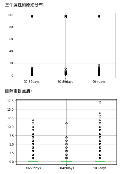
Manual processing is performed for three attributes with too concentrated values

#For three attributes whose values are too concentrated, the values of the three quartiles are equal, and the outlier is used directly_ The processing function causes all values to be deleted
#Therefore, these three attributes are processed manually

features = ['NumberOfTime30-59DaysPastDueNotWorse','NumberOfTime60-89DaysPastDueNotWorse','NumberOfTimes90DaysLate']
features_labels = ['30-59days','60-89days','90+days']
print('The original distribution of the three attributes:')
data[features].boxplot()
plt.xticks([1,2,3],features_labels)
plt.savefig('Original distribution of three attributes', dpi = 300 ,bbox_inches = 'tight')
plt.show()

print('After deleting outliers:')
data = data[data['NumberOfTime30-59DaysPastDueNotWorse']<90]
data = data[data['NumberOfTime60-89DaysPastDueNotWorse']<90]
data = data[data['NumberOfTimes90DaysLate']<90]

data[features].boxplot()
plt.xticks([1,2,3],features_labels)
plt.savefig('Distribution of three attributes after sorting', dpi = 300 ,bbox_inches = 'tight')
plt.show()
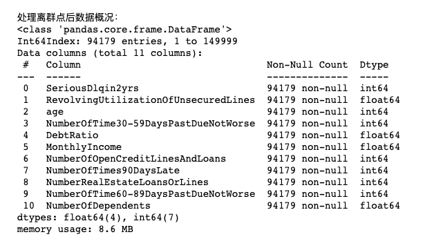
print('Data overview after processing outliers:')
data.info()

#Generate data sets and test sets
from sklearn.model_selection import train_test_split
#The original value 0 is normal and 1 is default. Because it is customary that the higher the credit score, the less likely the default is, so replace the original values of 0 and 1
data['SeriousDlqin2yrs'] = 1-data['SeriousDlqin2yrs']
Y = data['SeriousDlqin2yrs']
X = data.iloc[:,1:]

#Split training set and data set
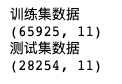
X_train,X_test,Y_train,Y_test = train_test_split(X,Y,test_size=0.3,random_state = 0)

train = pd.concat([Y_train,X_train],axis = 1)
test = pd.concat([Y_test,X_test],axis = 1)
clasTest = test.groupby('SeriousDlqin2yrs')['SeriousDlqin2yrs'].count()
print('Training set data')
print(train.shape)
print('Test set data')
print(test.shape)

III Attribute selection
In addition to excluding attributes with small absolute value by correlation analysis, the importance of an attribute on the target variable can be investigated through two indicators: WoE(Weight of Evidence): indication weight and IV(Information Value): information value, so as to determine the choice of attributes.

The calculation formula of these two indicators is as follows:
WoE = In(pctlGood/pctlBad)
MIV = WoE*(pctlGood-pctlBad)
IV = ∑ MIV

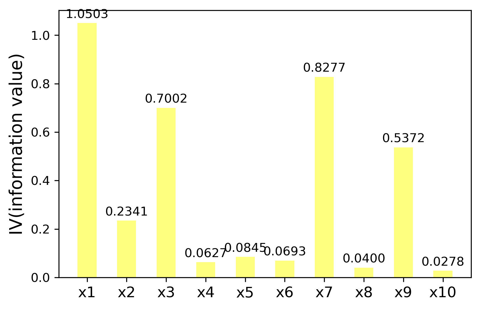
The relationship between the value of information value IV and the target variable to be studied is:
0 < IV < 0.02 extremely weak
0.02 < = IV < 0.1 weak
0.1 < = IV < 0.03 general
0.3 < = IV < 0.5 strong
0.5 < = IV < 1.0 very strong

#Box the attributes and calculate the values of WOE and IV

#Box the attributes and calculate the values of WOE and IV
def mono_bin(res,feat,n = 10):
    good = res.sum()
    bad = res.count()-good
    d1 = pd.DataFrame({'feat':feat,'res':res,'Bucket':pd.cut(feat,n)})
    d2 = d1.groupby('Bucket',as_index = True)
    d3 = pd.DataFrame(d2.feat.min(),columns = ['min'])
    d3['min'] = d2.min().feat
    d3['max'] = d2.max().feat
    d3['sum'] = d2.sum().res
    d3['total'] = d2.count().res
    d3['rate'] = d2.mean().res
    d3['woe'] = np.log((d3['rate']/(1-d3['rate']))/(good/bad))
    d3['goodattribute'] = d3['sum']/good
    d3['badattribute'] = (d3['total']-d3['sum'])/bad
    iv = ((d3['goodattribute']-d3['badattribute'])*d3['woe']).sum()
    d4 = (d3.sort_values(by = 'min'))
    cut = []
    cut.append(float('-inf'))
    for i in range(1,n):
        qua = feat.quantile(i/(n))
        cut.append(round(qua,4))
    cut.append(float('inf'))
    woe = list(d4['woe'].round(3))
    return d4,iv,cut,woe

def self_bin(res,feat,cat):
    good = res.sum()
    bad = res.count()-good
    d1 = pd.DataFrame({'feat':feat,'res':res,'Bucket':pd.cut(feat,cat)})
    d2 = d1.groupby('Bucket',as_index = True)
    d3 = pd.DataFrame(d2.feat.min(),columns = ['min'])
    d3['min'] = d2.min().feat
    d3['max'] = d2.max().feat
    d3['sum'] = d2.sum().res
    d3['total'] = d2.count().res
    d3['rate'] = d2.mean().res
    d3['woe'] = np.log((d3['rate']/(1-d3['rate']))/(good/bad))
    d3['goodattribute'] = d3['sum']/good
    d3['badattribute'] = (d3['total']-d3['sum'])/bad
    iv = ((d3['goodattribute']-d3['badattribute'])*d3['woe']).sum()
    d4 = (d3.sort_values(by = 'min'))
    woe = list(d4['woe'].round(3))
    return d4,iv,woe

Each attribute is divided into boxes according to the specified interval. cutx3/6/7/8/910 boxes are defined here

pinf = float('inf')
ninf = float('-inf')
dfx1,ivx1,cutx1,woex1 = mono_bin(train['SeriousDlqin2yrs'],train['RevolvingUtilizationOfUnsecuredLines'],n = 10)
#Display the information of revolutionutilizationofunsecure lines and WOE
print('='*60)
print('display RevolvingUtilizationOfUnsecuredLines Sub box and WOE information:')
print(dfx1)
dfx2,ivx2,cutx2,woex2 = mono_bin(train['SeriousDlqin2yrs'],train['age'],n = 10)
dfx4,ivx4,cutx4,woex4 = mono_bin(train['SeriousDlqin2yrs'],train['DebtRatio'],n = 10)
dfx5,ivx5,cutx5,woex5 = mono_bin(train['SeriousDlqin2yrs'],train['MonthlyIncome'],n = 10)
#Divide the data of 3, 6, 7, 8, 9 and 10 columns into boxes at specified intervals
cutx3 = [ninf,0,1,3,5,pinf]
cutx6 = [ninf,1,2,3,5,pinf]
cutx7 = [ninf,0,1,3,5,pinf]
cutx8 = [ninf,0,1,2,3,pinf]
cutx9 = [ninf,0,1,3,pinf]
cutx10 = [ninf,0,1,2,3,5,pinf]

#Divide the numberoftime30-59dayspastduenotword attribute into 5 segments according to the interval specified by cutx3
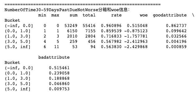
dfx3,ivx3,woex3 = self_bin(train['SeriousDlqin2yrs'],train['NumberOfTime30-59DaysPastDueNotWorse'],cutx3)
#Display NumberOfTime30-59DaysPastDueNotWorse distribution box and woe information:
print('='*60)
print('NumberOfTime30-59DaysPastDueNotWorse Sub box and woe Information:')
print(dfx3)
dfx6,ivx6,woex6 = self_bin(train['SeriousDlqin2yrs'],train['NumberOfOpenCreditLinesAndLoans'],cutx6)
dfx7,ivx7,woex7 = self_bin(train['SeriousDlqin2yrs'],train['NumberOfTimes90DaysLate'],cutx7)
dfx8,ivx8,woex8 = self_bin(train['SeriousDlqin2yrs'],train['NumberRealEstateLoansOrLines'],cutx8)
dfx9,ivx9,woex9 = self_bin(train['SeriousDlqin2yrs'],train['NumberOfTime60-89DaysPastDueNotWorse'],cutx9)
dfx10,ivx10,woex10 = self_bin(train['SeriousDlqin2yrs'],train['NumberOfDependents'],cutx10)

Draw the calculated IV attribute

#Select properties by iv
ivlist = [ivx1,ivx2,ivx3,ivx4,ivx5,ivx6,ivx7,ivx8,ivx9,ivx10]
index = ['x1','x2','x3','x4','x5','x6','x7','x8','x9','x10']
fig1 = plt.figure(1)
ax1 = fig1.add_subplot(1,1,1)
x = np.arange(len(index))+1
ax1.bar(x,ivlist,width = 0.48,color = 'yellow',alpha = 0.5)
ax1.set_xticks(x)
ax1.set_xticklabels(index,rotation = 0,fontsize = 12)
ax1.set_ylabel('IV(information value)',fontsize = 14)
for a,b in zip(x,ivlist):
    plt.text(a,b+0.01,'%.4f'%b,ha = 'center',va = 'bottom',fontsize = 10)
plt.savefig('iv Value.png', dpi = 300,bbox_inches = 'tight')
plt.show()

IV Model training stage
Get defined_ The WoE function is used to convert the original data into WoE values to improve the training results of the model. Call get_wor function, which converts the attributes of training set and test set into WoE value

#Model training stage
#Find the corresponding value of the attribute woe
def get_woe(feat,cut,woe):
    res = []
    for row in feat.iteritems():
        value = row[1]
        j = len(cut)-2
        m = len(cut)-2
        while j>=0:
            if value>=cut[j]:
                j=-1
            else:
                j-=1
                m-=1
        res.append(woe[m])
    return res
#Call get_ The woe function converts the attribute values of the training set and the test set into woe values respectively
woe_train = pd.DataFrame()
woe_train['SeriousDlqin2yrs'] = train['SeriousDlqin2yrs']
woe_train['RevolvingUtilizationOfUnsecuredLines'] = get_woe(train['RevolvingUtilizationOfUnsecuredLines'], cutx1, woex1)
woe_train['age'] = get_woe(train['age'], cutx2, woex2)
woe_train['NumberOfTime30-59DaysPastDueNotWorse'] = get_woe(train['NumberOfTime30-59DaysPastDueNotWorse'], cutx3, woex3)
woe_train['DebtRatio'] = get_woe(train['DebtRatio'], cutx4, woex4)
woe_train['MonthlyIncome'] = get_woe(train['MonthlyIncome'], cutx5, woex5)
woe_train['NumberOfOpenCreditLinesAndLoans'] = get_woe(train['NumberOfOpenCreditLinesAndLoans'], cutx6, woex6)
woe_train['NumberOfTimes90DaysLate'] = get_woe(train['NumberOfTimes90DaysLate'], cutx7, woex7)
woe_train['NumberRealEstateLoansOrLines'] = get_woe(train['NumberRealEstateLoansOrLines'], cutx8, woex8)
woe_train['NumberOfTime60-89DaysPastDueNotWorse'] = get_woe(train['NumberOfTime60-89DaysPastDueNotWorse'], cutx9, woex9)
woe_train['NumberOfDependents'] = get_woe(train['NumberOfDependents'], cutx10, woex10)     

#Replace the attributes of the test set with woe     
woe_test = pd.DataFrame()
woe_test['SeriousDlqin2yrs'] = train['SeriousDlqin2yrs']
woe_test['RevolvingUtilizationOfUnsecuredLines'] = get_woe(train['RevolvingUtilizationOfUnsecuredLines'], cutx1, woex1)
woe_test['age'] = get_woe(train['age'], cutx2, woex2)
woe_test['NumberOfTime30-59DaysPastDueNotWorse'] = get_woe(train['NumberOfTime30-59DaysPastDueNotWorse'], cutx3, woex3)
woe_test['DebtRatio'] = get_woe(train['DebtRatio'], cutx4, woex4)
woe_test['MonthlyIncome'] = get_woe(train['MonthlyIncome'], cutx5, woex5)
woe_test['NumberOfOpenCreditLinesAndLoans'] = get_woe(train['NumberOfOpenCreditLinesAndLoans'], cutx6, woex6)
woe_test['NumberOfTimes90DaysLate'] = get_woe(train['NumberOfTimes90DaysLate'], cutx7, woex7)
woe_test['NumberRealEstateLoansOrLines'] = get_woe(train['NumberRealEstateLoansOrLines'], cutx8, woex8)
woe_test['NumberOfTime60-89DaysPastDueNotWorse'] = get_woe(train['NumberOfTime60-89DaysPastDueNotWorse'], cutx9, woex9)
woe_test['NumberOfDependents'] = get_woe(train['NumberOfDependents'], cutx10, woex10)      

import statsmodels.api as sm
from sklearn.metrics import roc_curve,auc

Y = woe_train['SeriousDlqin2yrs']
X = woe_train.drop(['SeriousDlqin2yrs','DebtRatio','MonthlyIncome','NumberOfOpenCreditLinesAndLoans','NumberRealEstateLoansOrLines','NumberOfDependents'],axis = 1)
X1 = sm.add_constant(X)
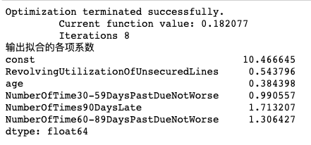
logit = sm.Logit(Y,X1)
Logit_model = logit.fit()
print('Output fitting coefficients')
print(Logit_model.params)

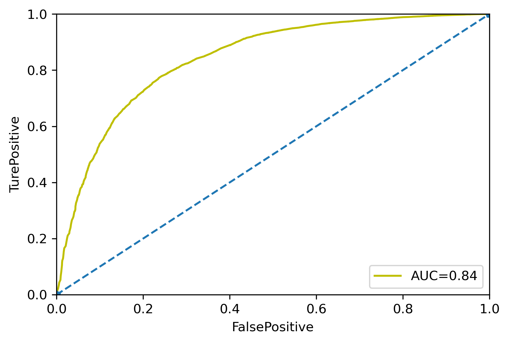
Draw the AUC curve of the model

Y_test = woe_test['SeriousDlqin2yrs']
X_test = woe_test.drop(['SeriousDlqin2yrs','DebtRatio','MonthlyIncome',
                        'NumberOfOpenCreditLinesAndLoans',
                        'NumberRealEstateLoansOrLines','NumberOfDependents'],axis=1)
X3 = sm.add_constant(X_test)
resu = Logit_model.predict(X3)
fpr,tpr,threshold = roc_curve(Y_test,resu)
rocauc = auc(fpr,tpr)
plt.plot(fpr,tpr,'y',label='AUC=%0.2f' % rocauc)
plt.legend(loc='lower right')
plt.plot([0,1],[0,1],'p--')
plt.xlim([0,1])
plt.ylim([0,1])
plt.ylabel('TurePositive')
plt.xlabel('FalsePositive')
plt.savefig('Model AUC curve.png',dpi=300,bbox_inches='tight')
print('Model AUC Curve:')
plt.show()

#Define get_ The score function is used to calculate the basic score of each sub box
def get_score(coe,woe,factor):
    scores = []
    for w in woe:
        score = round(coe*w*factor,0)
        scores.append(score)
    return scores
#Define compte_score function to calculate the basic score corresponding to the specific attribute value
def compute_score(feat,cut,score):
    res = []
    for row in feat.iteritems():
        value = row[1]
        j = len(cut)-2
        m = len(cut)-2
        while j>=0:
            if value>=cut[j]:
                j=-1
            else:
                j-=1
                m-=1
        res.append(score[m])
    return res
import math
coe = Logit_model.params
p = 20/math.log(2)
q = 600-20*math.log(20)/math.log(2)
baseScore = round(q+p*coe[0],0)

x1 = get_score(coe[1],woex1,p)
print('The attribute value in column 1 is the score corresponding to each sub box section')
print(x1)

x2 = get_score(coe[2],woex2,p)
x3 = get_score(coe[3],woex3,p)
x7 = get_score(coe[4],woex7,p)
x9 = get_score(coe[5],woex9,p)

#print(x2)
#print(x3)
#print(x3)
#Calculate score
test['BaseScore'] = np.zeros(len(test))+baseScore
test['x1'] = compute_score(test['RevolvingUtilizationOfUnsecuredLines'],cutx1,x1)
test['x2'] = compute_score(test['age'],cutx2,x2)
test['x3'] = compute_score(test['NumberOfTime30-59DaysPastDueNotWorse'],cutx3,x3)
test['x7'] = compute_score(test['NumberOfTimes90DaysLate'],cutx7,x7)
test['x9'] = compute_score(test['NumberOfTime60-89DaysPastDueNotWorse'],cutx9,x9)

test['Score'] = test['x1']+test['x2']+test['x3']+test['x7']+test['x9']+baseScore

The attribute value in column 1 is the score corresponding to each sub box section
[20.0, 10.0, 4.0, -2.0, -7.0, -13.0, -19.0, -21.0, -41.0, -38.0]

Normal = test.loc[test['SeriousDlqin2yrs']==1]
Charged = test.loc[test['SeriousDlqin2yrs']==0]

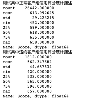
print('Statistical description of credit scores of normal customer groups in the test set')
print(Normal['Score'].describe())
print('Statistical description of credit score of default customer group in the test set')
print(Charged['Score'].describe())

import seaborn as sns
plt.figure(figsize = (10,4))
sns.kdeplot(Normal['Score'],label = 'normal',linewidth = 2,linestyle = '--')
sns.kdeplot(Charged['Score'],label = 'charged',linewidth = 2,linestyle = '-')
plt.xlabel('Score',fontdict = {'size':10})
plt.ylabel('probability',fontdict = {'size':10})
plt.title('normal/charged',fontdict={'size':18})
plt.savefig('Credit distribution of default and normal customers.png',dpi = 300,bbox_inches = 'tight')
plt.show()

Credit score distribution of defaulting customers and normal customers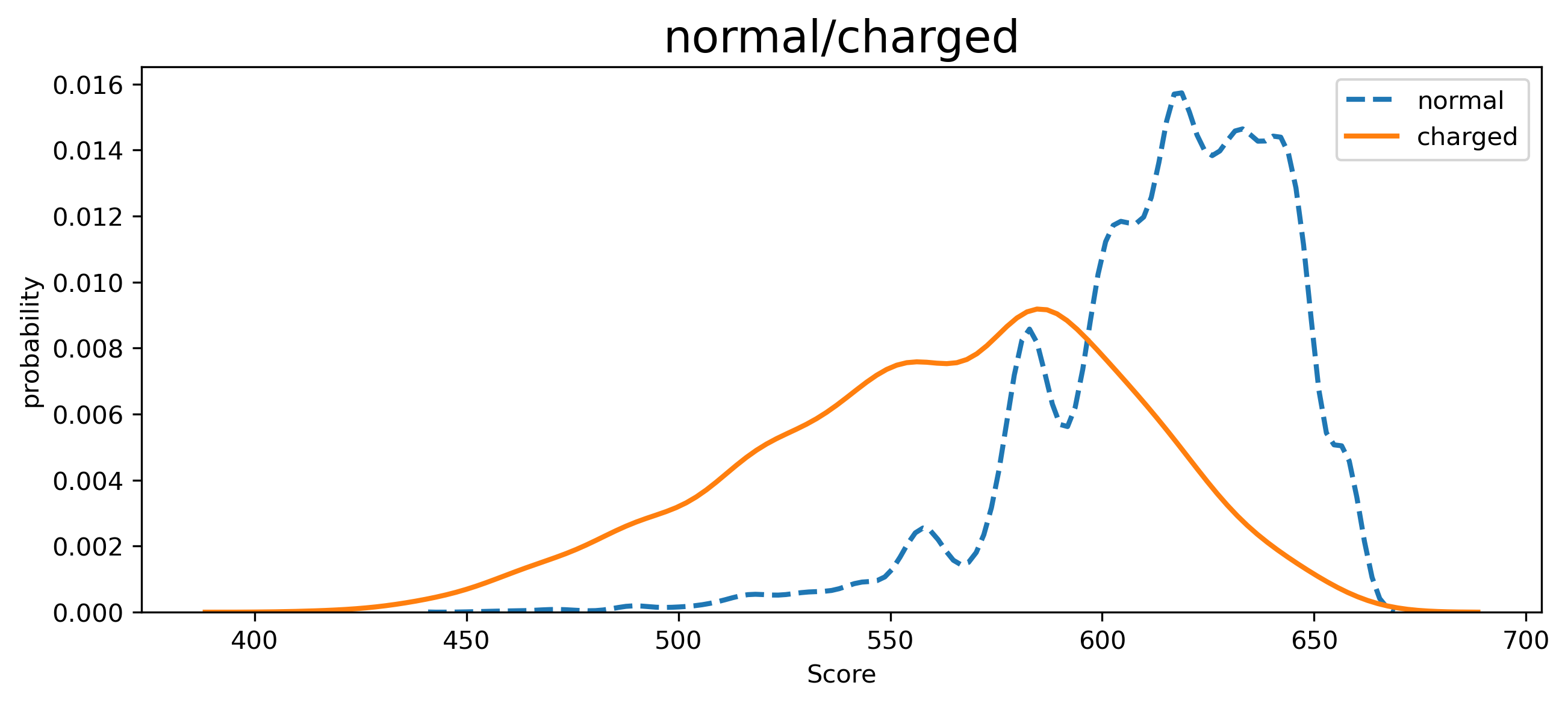

Apply the trained model to customer credit scoring

#Apply the trained model to customer credit scoring
cusInfo = {'RevolvingUtilizationOfUnsecuredLines':0.248537,'age':48,'NumberOfTime30-59DaysPastDueNotWorse':0,
           'NumberOfTime60-89DaysPastDueNotWorse':0,'DebtRatio':0.177586,'MonthlyIncome':4166,
           'NumberOfOpenCreditLinesAndLoans':11,'NumberOfTimes90DaysLate':0,'NumberRealEstateLoansOrLines':1,
           'NumberOfTime60-89DaysPastDueNotWorse':0,'NumberOfDependents':0}
custData = pd.DataFrame(cusInfo,pd.Index(range((1))))
custData.drop(['DebtRatio','MonthlyIncome','NumberOfOpenCreditLinesAndLoans','NumberRealEstateLoansOrLines','NumberOfDependents'],axis = 1)

custData['x1'] = compute_score(custData['RevolvingUtilizationOfUnsecuredLines'], cutx1,x1)
custData['x2'] = compute_score(custData['age'], cutx2,x2)
custData['x3'] = compute_score(custData['NumberOfTime30-59DaysPastDueNotWorse'], cutx3,x3)
custData['x7'] = compute_score(custData['NumberOfTimes90DaysLate'], cutx7,x7)
custData['x9'] = compute_score(custData['NumberOfTime60-89DaysPastDueNotWorse'], cutx9,x9)

custData['Score'] = custData['x1']+custData['x2']+custData['x3']+custData['x7']+custData['x9']+baseScore
print('The customer's credit score is:')
print(custData.loc[0,'Score'])             

The customer's credit score is:
613.0