CS131 learning notes #0

1. Introduction to numpy

The essence of image recognition processing is matrix operation. python's numpy library performs this kind of operation, so learning numpy is a necessary step before image learning.

import numpy as np is usually used to use the numpy package

1.1 general creation method of matrix

• Cannot create an empty array
• General method of creating array: y = NP array([[1,2,3,4,5], [6,7,8,9,10]])
• Read size: y.shape
• Create zero matrix: NP Zero ((3,3)) # creates a 0 matrix with a size of 3 * 3
• Create unit array: identity = NP identity(3)
• Create all one matrix: ones = NP ones((2,2))

1.2 Broadcasting and NP Use of mean

import numpy as np
#If we want to adjust the row average of any matrix to 0:
matrix = 10*np.random.rand(4,5)
row_means = matrix.mean(axis = 1).reshape((4,1))
matrix = matrix - row_means
print(matrix)
#axis does not set a value, calculates the mean value of m*n numbers, and returns a real number
#axis = 0: compress rows and calculate the mean value of each column
#axis =1: compress the column and calculate the average value of each row

1.3 numpy.random usage

• numpy. random. Random use

#Three parameters: low, high and size. The default high is None. If there is only low, the range is [0, low]. If there is high, the range is [low,high).
#Returns a random integer in a semi open interval [low, high].
>>> np.random.randint(2, size=10)
array([1, 0, 0, 0, 1, 1, 0, 0, 1, 0])

>>> np.random.randint(1, size=10)
array([0, 0, 0, 0, 0, 0, 0, 0, 0, 0])

>>> np.random.randint(5, size=(2, 4))
array([[4, 0, 2, 1],
       [3, 2, 2, 0]])

• numpy.random.rand use

#This function can return one or a group of random sample values subject to "0 ~ 1" uniform distribution. The value range of random samples is [0,1], excluding 1. 
>>> np.random.rand(3,2)
array([[ 0.14022471,  0.96360618],  
       [ 0.37601032,  0.25528411],  
       [ 0.49313049,  0.94909878]]) 

• numpy.random.randn usage

#The randn function returns one or a set of samples with a standard normal distribution.
np.random.randn(2,4)
array([[ 0.27795239, -2.57882503,  0.3817649 ,  1.42367345],
      [-1.16724625, -0.22408299,  0.63006614, -0.41714538]])
#standard normal distribution
#The standard normal distribution, also known as u distribution, is a normal distribution with 0 as the mean and 1 as the standard deviation, which is recorded as N (0,1).

1.4 use of Boolean masks

• Basic judgment

import numpy as np
array = np.array(range(20)).reshape((4,5))#Matrix of 4 * 5,1-20
print(array)

output = array > 10
output
#out: 
array([[False, False, False, False, False],
       [False, False, False, False, False],
       [False,  True,  True,  True,  True],
       [ True,  True,  True,  True,  True]])

array[output]
#out: 
array([11, 12, 13, 14, 15, 16, 17, 18, 19])

#Multiple judgments can be made
mask = (array < 5) | (array > 15)
#mask = array < 5 | array > 15
mask
#out: 
array([[ True,  True,  True,  True,  True],
       [False, False, False, False, False],
       [False, False, False, False, False],
       [False,  True,  True,  True,  True]])

• Practical application

#Given a matrix, change all of the negative values to zero
matrix = 2*np.random.rand(5, 5) - 1#(- 1,1) uniformly distributed random matrix
### SOLUTION ###
mask = matrix < 0
print(mask)
matrix[mask] = 0#Assign all values in the mask to 0
print(matrix)

1.5 reshape usage

#when your reshape, by default you fill the new array by rows
x = np.linspace(1, 12, 6)
print(x)
#[ 1.   3.2  5.4  7.6  9.8 12. ]

x = x.reshape((3,2)) #does not reshape in place!
print(x)
#[[ 1.   3.2]
# [ 5.4  7.6]
# [ 9.8 12. ]]

print(x.reshape(-1))#-1 is equivalent to the default value and will be calculated automatically by the system
[ 1.   3.2  5.4  7.6  9.8 12. ]

print(x.reshape(2,-1))
[[ 1.   3.2  5.4]
 [ 7.6  9.8 12. ]]

1.6 numpy deep copy

We find that the matrix assignment in numpy is a shallow copy, and the copy is the address, for example:

array = np.linspace(1, 10, 10)
array
#out
#array([ 1.,  2.,  3.,  4.,  5.,  6.,  7.,  8.,  9., 10.])

dup = array
dup
#out
#array([ 1.,  2.,  3.,  4.,  5.,  6.,  7.,  8.,  9., 10.])

array[0] = 100
dup
#out
#array([100.,  2.,  3.,  4.,  5.,  6.,  7.,  8.,  9.,  10.])

print(id(array))
print(id(dup))
#out
#120645422176
#120645422176

It can be seen that after using '=' assignment, the addresses pointed to by array and dup are the same, so modifying one of them and the other will also change. To avoid this situation, we use numpy's deep copy method.

#using copy
import copy
array = np.linspace(1, 10, 10)
dup = copy.deepcopy(array)
#It can also be written here as DUP = NP Copy (array) or DUP = array copy()
print(id(array))
print(id(dup))
array[0] = 100
dup

120649253152
120664256640
array([ 1.,  2.,  3.,  4.,  5.,  6.,  7.,  8.,  9., 10.])

Error method: using slicing syntax [:]

#slicing
array = np.linspace(1, 10, 10)
dup = array[:]
print(id(array))
print(id(dup))
array[0] = 100
dup

2552119240816
2552119240336
[100.   2.   3.   4.   5.   6.   7.   8.   9.  10.]

We found that although the addresses are different, the values of dup and array change together

2. Introduction to pyplot

2.1 pyplot

import matplotlib.pyplot as plt

x = np.arange(10)**2
print(x)
plt.plot(x)
plt.show()

The output table is as follows:

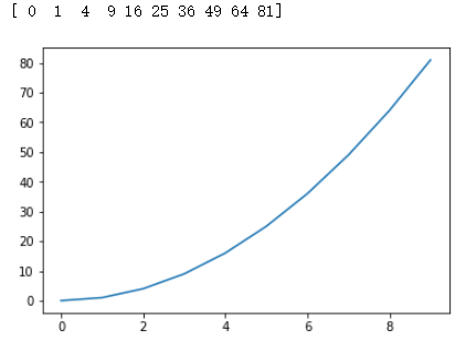
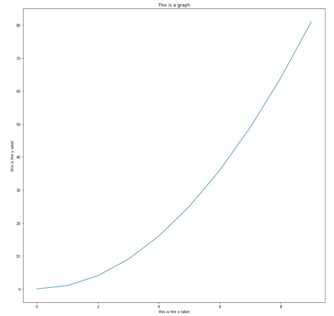
Of course, many details can be added:

plt.figure(figsize = (15,15))
plt.plot(x)
plt.title("This is a graph")
plt.xlabel("this is the x label")
plt.ylabel("this is the y label")
plt.show()

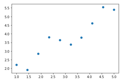
2.2 scatter diagram

x = np.concatenate((np.linspace(1, 5, 10).reshape(10, 1), np.ones(10).reshape(10, 1)), axis = 1)
print(x)
y = x[:,0].copy() + 2*np.random.rand(10) - 0.5
print(y)
plt.scatter(x[:,0], y)#Scatter diagram

3. Image reading

3.1 basic composition of pictures

As we all know, an image is composed of three RGB color layers. For an image, We can use the matrix of (h,w,3), where h and w represent the height and width of the picture respectively, and 3 represents three basic color channels. The number stored in the corresponding matrix of each color channel represents the gray value of the color light, and the pixels composed of three different gray colors are spliced into a colorful image.

The gray value is not the literal "black-and-white" value, but refers to the brightness value of a color. For example, a layer (400300, 1) of the picture represents the red channel matrix, in which the red gray value is stored.

Each color channel stores its corresponding gray value. The gray value of the last three layers of channels is like color matching. Once adjusted, the desired color in the picture can be called out according to the gray value of different colors in the three primary colors.

Take any point as shown in the figure. When displaying, put the red gray value of the point into channel R, the green gray value into channel G and the blue gray value into channel B. the three gray information can call out the corresponding color like color matching.

In general, channels represent channels of different colors. (of course, there are some special channels, such as alpha channel, which stores picture transparency information.) gray value represents the brightness of a color.

3.2 code implementation of picture reading

def display(img):
    plt.figure(figsize = (5,5))
    plt.imshow(img)#display picture
    plt.axis('off')#Do not display axes
    plt.show() 
def load(image_path):
    out = io.imread(image_path)
    #Read the picture. The second parameter defaults to False. When it is True, it is a grayscale image
    out = out.astype(np.float64) / 255
    return out

from skimage import io
img = load('image1.jpg')
display(img)

def rgb_exclusion(image, channel):
    out = image.copy()
    if channel == 'R':
        out[:, :, 0] = 0
    elif channel == 'G':
        out[:, :, 1] = 0
    elif channel == 'B':
        out[:, :, 2] = 0
    return out#Turn off one of the RGB channels

Note: scikit image is an image processing package based on scipy. It processes pictures as numpy arrays. It is a very good digital image processing tool to be learned later. The following table is for reference.

Sub module name	Main functions
io	Read, save, and display pictures or videos
data	Provide some test pictures and sample data
color	Color space transformation
filters	Image enhancement, edge detection, sorting filter, automatic threshold, etc
draw	Basic graphics drawing on numpy array, including lines, rectangles, circles and text
transform	Geometric transformation or other transformations, such as rotation, stretching, radon transformation, etc
morphology	Morphological operations, such as opening and closing operations, skeleton extraction, etc
exposure	Image intensity adjustment, such as brightness adjustment, histogram equalization, etc
feature	Feature detection and extraction, etc
measure	Measurement of image attributes, such as similarity or contour lines
segmentation	image segmentation
restoration	image restoration
util	General function

reference resources

https://zhuanlan.zhihu.com/p/360220467

https://www.jianshu.com/p/be7af337ffcd

4. Linear algebra

4.1 solving linear equations:

For example, say we wanted to solve the linear system
A x = b Ax=b Ax=b

A = np.array([[1, 1], [2, 1]])
b = np.array([[1], [0]])
#This function takes parameters A, b, and returns x such that Ax =b. 
x = np.linalg.solve(A, b)

4.2 best fit:

Linear regression finds the "line of best fit" by minimizing the residual sum of squares.

If we have n datapoints { ( x 1 , y 1 ) , . . . , ( x n , y n ) } \{(x_1, y_1), ... ,(x_n, y_n)\} {(x1​,y1​),...,(xn​,yn​)}​, the objective function takes the form l o s s ( X ) = Σ i = 1 n ( y i − f ( x i ) ) 2 loss(X) = \Sigma_{i = 1}^n (y_i - f(x_i))^2 loss(X)=Σi=1n​(yi​−f(xi​))2​ where f ( x i ) = θ 0 + θ 1 x 1 + . . . + θ n x n f(x_i) = \theta_0 + \theta_1 x_1 + ... +\theta_n x_n f(xi​)=θ0​+θ1​x1​+...+θn​xn​​

It turns out the parameters such that the loss function is minimized are given by the closed form solution θ = ( X T X ) − 1 X T y \theta = (X^T X)^{-1} X^T y θ=(XTX)−1XTy​

​

For this algorithm, let's review the least squares method in Linear Algebra:

For errors: E ( x ) = ∣ ∣ b − A x ∣ ∣ 2 E(x)=||b-Ax||^2 E(x) = ∣∣ b − Ax ∣∣ 2, find x to minimize e, where A is the column full rank matrix and p is the projection of b on the column space A.

By Pythagorean theorem:

∣ ∣ A x − p ∣ ∣ 2 + ∣ ∣ b − p ∣ ∣ 2 = ∣ ∣ b − A x ∣ ∣ 2 || Ax-p||^2+||b-p||^2=||b-Ax||^2 ∣∣Ax−p∣∣2+∣∣b−p∣∣2=∣∣b−Ax∣∣2

For any b:

∣ ∣ b − A x ∣ ∣ 2 ≥ ∣ ∣ b − p ∣ ∣ 2 ||b-Ax||^2 \geq ||b-p||^2 ∣∣b−Ax∣∣2≥∣∣b−p∣∣2

Therefore, E takes the minimum value if and only if x is obtained so that A x = p Ax=p Ax=p. because column A is full rank, the equation has a unique solution:

x ^ = ( A T A ) − 1 A T b \hat{x} = (A^TA)^{-1}A^Tb x^=(ATA)−1ATb

Next, let's do some practical operations with python

First get some points

x = np.concatenate((np.linspace(1, 5, 10).reshape(10, 1), np.ones(10).reshape(10, 1)), axis = 1)#axis=1 indicates splicing by column
print(x)
y = x[:,0].copy() + 2*np.random.rand(10) - 0.5
print(y)
plt.scatter(x[:,0], y)
plt.show()

Find the coefficient θ \theta θ

theta = np.linalg.lstsq(x, y, rcond=None)[0]
#Least square is solved by using built-in functions
print(theta)

​ [0.72037691 1.55604653]

Or:

theta = np.linalg.inv(x.T.dot(x)).dot(x.T).dot(y)
#Using the formula to solve the minimum second pass
print(theta)

The same result is obtained: [0.72037691 1.55604653]

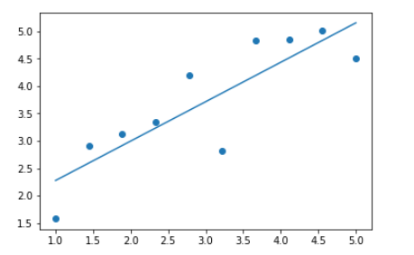
Finally, draw a straight line:

plt.scatter(x[:,0], y)
plt.plot(x[:,0], x[:,0]*theta[0] + theta[1])