Introduction: Using the area of the ring to calculate the radius of the circle in reverse, a more stable radius of the circle can be obtained. For the movement of the standard template on the scanner, you can see the change law of the corresponding measurement results. The following is a preliminary analysis of such changes.
Key words: bacteriostatic circle measuring instrument, OpenCV, contour
§ 01 image preprocessing
in scanner based Bacteriostatic circle In the measuring instrument, the drug performance is evaluated according to the size of the bacteriostatic circle formed by bacteriostatic drugs in the picture. The current standard is to describe it by its diameter.

due to the moving process in the measurement process:
- Measure the placement of bacteria tray;
- Scanner movement, etc;
image distortion will appear in the process of obtaining the picture. In order to avoid the influence of this distortion on the measurement results, it is necessary to test the corresponding distortion of the adopted mechanical structure through the calibrated metal template.
in Get pictures of different positions of checkerboard and standard template on the scanner The scanning pictures of the metal template of the bacteriostatic ring sprayed with yellow paint at different positions and heights above were obtained. The performance of scanner for image acquisition process is studied through the following algorithm.
in the early stage, the relative position of the metal template has been obtained through HoughCircles in OpenCV. Because the accuracy of the position and size obtained by HoughCircles is not high, it is necessary to use other super-resolution methods to obtain the estimation of the ring radius of the metal bacteriostatic ring.
1.1 pre extraction of ring position
in order to improve the calculation speed, the collected pictures are preprocessed below.
1.1.1 extraction method
there are two ways of pretreatment:
- Obtain the specific position of each ring;
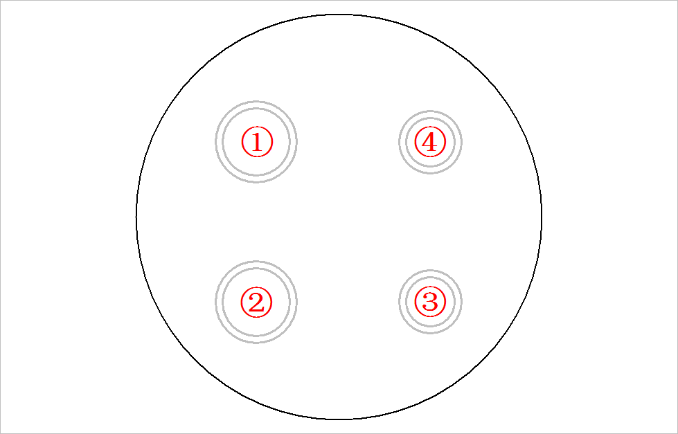
- Pre sort rings by Get pictures of different positions of checkerboard and standard template on the scanner In the way given in, there are four rings [large, large, small and small] along the counterclockwise direction.
(1) Preprocessing algorithm
from headm import *                 # =
import cv2
from tqdm import tqdm

scandiagblock = '/home/aistudio/work/Scanner/ScanDiagBlock'
scanrowblock = '/home/aistudio/work/Scanner/ScanRowBlock'
scanvertblock = '/home/aistudio/work/Scanner/ScanVertBlock'
scandir = '/home/aistudio/work/Scanner'

filedir = scanrowblock
npzfile = os.path.join(scandir, os.path.basename(filedir)+'.npz')

filedim = sorted([s for s in os.listdir(filedir) if s.find("jpg") > 0])

def sortcircles(cc):
    cca = mean(cc[0], axis=0)

    angle = [math.atan2(c[1]-cca[1], c[0]-cca[0])*180/pi for c in cc[0]]
    angle = [s if s >= 0 else 360+s for s in angle]

    ar = sorted(zip(angle, cc[0].T[2], cc[0]))
    sortr = [s[1] for s in ar]
    rcompare = list(array(sortr) > 100)
    ccc = [s[2] for s in ar]

    for i in range(3):
        rc = roll(rcompare, i+1)
        rsr = roll(sortr, i+1)
        cccr = roll(ccc, i + 1, axis=0)

        if rc[0] == True and rc[1] == True:
            break

    return rsr, cccr

def modelArg(filename):
    img = cv2.imread(os.path.join(filedir, filename))
    gray = cv2.cvtColor(img, cv2.COLOR_BGR2GRAY)
    circles = cv2.HoughCircles(gray, cv2.HOUGH_GRADIENT, 1, 50,
                               param1=150, param2=40,
                               minRadius=90, maxRadius=115)
    bigcircle = cv2.HoughCircles(gray, cv2.HOUGH_GRADIENT, 1, 50,
                                 param1=200, param2=60,
                                 minRadius=530, maxRadius=580)

    cc = []
    bcx = bigcircle[0][0][0]
    bcy = bigcircle[0][0][1]
    bcr = bigcircle[0][0][2]

    for c in circles[0]:
        cx = c[0]
        cy = c[1]

        dist = sqrt((cx-bcx)**2 + (cy-bcy)**2)
        if dist < bcr*0.75 and c[0] <900:
            cc.append(c)

    return img, array([cc])

gifpath = '/home/aistudio/GIF'
if not os.path.isdir(gifpath):
    os.makedirs(gifpath)
gifdim = os.listdir(gifpath)
for f in gifdim:
    fn = os.path.join(gifpath, f)
    if os.path.isfile(fn):
        os.remove(fn)

alldim = []
allfile = []
for id,f in tqdm(enumerate(filedim)):
    img,c = modelArg(f)
    cc,cccr = sortcircles(c)

    alldim.append(cccr)
    allfile.append(os.path.join(filedir, f))

    img[where(img<50)] =0
    for ccc in cccr:
        cv2.circle(img, (ccc[0], ccc[1]), int(ccc[-1]), (0,0,255), 10)

    plt.figure(figsize=(10,10))
    plt.imshow(img[:,:,::-1])
    savefile = os.path.join(gifpath, '%03d.jpg'%id)
    plt.savefig(savefile)
    plt.close()

    if len(c[0]) != 4:
        printt(c:)
        break
    else:
        pass

savez(npzfile, alldim=alldim, allfile=allfile)
1.1.2 extraction results
(1) Horizontal scanning picture
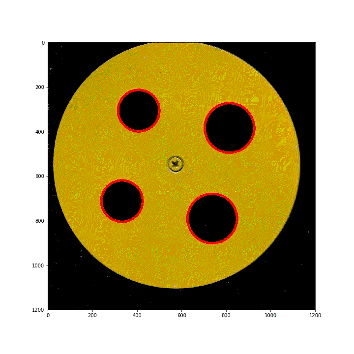
this is the cutting of the picture obtained by moving the ring horizontally for 50 steps. In the last picture, there was an error in detecting the small ring due to the interference of the background. After the actual correct picture, there are about 42 pictures in front.

(2) Diagonal scan
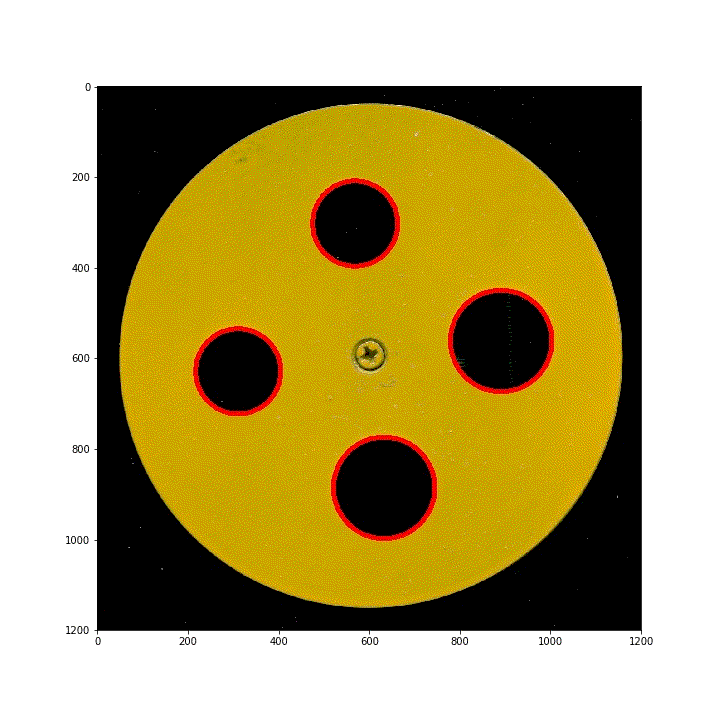
below are 100 scanned segmented images of images obtained by translating the ring along the diagonal of the scanner. Using HoughCircles, the position and order of the four rings have been preprocessed.
(3) Vertical lifting ring
lifting the ring template vertically will deform the picture badly. In the early stage, the parameters used in Hough transform can only adapt to the previous 13 pictures. The rest of the picture detection results can not meet the requirements. For this type of change, when determining the later image parameters, the first one will be used to detect the position of the four rings as the unified standard of processing.
§ 02 ring area
use the area of the ring S S S. Conversely, according to the circle S = π r 2 S = \pi r^2 S = π r2, which in turn defines the radius (diameter) of the ring.
2.1 calculate the area equivalent radius
2.1.1 obtain the ring boundary
zipfilediag = '/home/aistudio/work/Scanner/ScanDiagBlock.npz'
scandirdiag = '/home/aistudio/work/Scanner/ScanDiagBlock'
alldata = load(zipfilediag, allow_pickle=True)

alldim = alldata['alldim']
allfile = alldata['allfile']
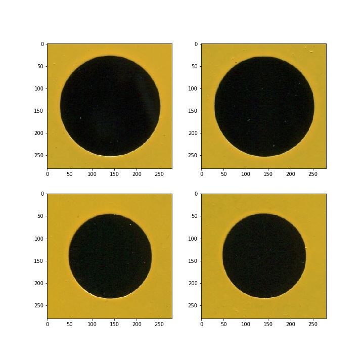
(1) Convert image to black and white
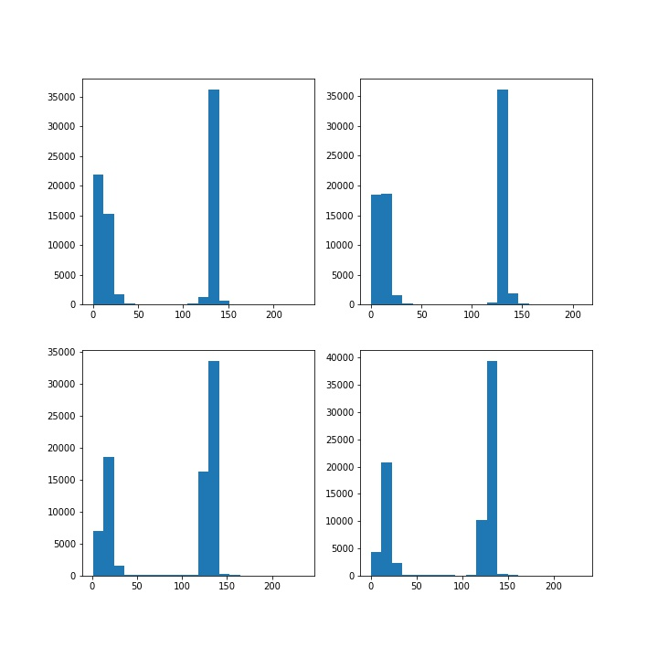
after converting into gray image, the brightness of pixels is counted. You can see the most appropriate threshold if binarization is performed t h r e s h = 70 thresh = 70 thresh=70 .
(2) Look for contours on black-and-white drawings

2.1.2 radius obtained by boundary
(1) Find the correct area
passed CV2 Contourarea() calculates the area of all Contours. You can see that the area of the circle should be the second largest area in the result.
areaDim: [77841.0, 39682.0, 0.5, 0.0]
areaDim: [77841.0, 39398.5, 1.0, 0.5, 0.0]
areaDim: [77841.0, 27712.0, 0.0, 0.0, 0.0, 1.0]
areaDim: [77841.0, 27963.5, 0.0, 0.0, 0.0, 0.0]
utilization r = A / π r = \sqrt {A/\pi } r=A/π Calculate the equivalent radius of the circle.
ratioDim: [112.38849097458859, 111.98630296072854, 93.92019785927417, 94.34542120474333]
2.1.3 diagonal translation formwork radius
(1)70
the circular metal template is translated diagonally on the scanner to obtain 100 moving pictures. Process all images to obtain all ring radii.
the variance and range corresponding to the four rings are given below:
std(rdim1): 0.09883722204508248
std(rdim2): 0.1129093828814647
std(rdim3): 0.25045297377194586
std(rdim4): 0.21107984867821605

max(rdim1)-min(rdim1): 0.4408802395310687
max(rdim2)-min(rdim2): 0.5670444141300806
max(rdim3)-min(rdim3): 1.0083621030471193
max(rdim4)-min(rdim4): 0.8065292585312562
(2) The threshold is set to 100
std(rdim1): 0.09900553310591087
std(rdim2): 0.11370717076338002
std(rdim3): 0.24494327932253113
std(rdim4): 0.20506054635254523

max(rdim1)-min(rdim1): 0.45511065871777134
max(rdim2)-min(rdim2): 0.5779160789730753
max(rdim3)-min(rdim3): 0.9834303156866042
max(rdim4)-min(rdim4): 0.8077211123899559
it can be seen from the above test that the change of binarization threshold will affect the size of the final calculated output.
2.1.4 horizontal translation processing results
std(rdim1): 0.07740474002858148
std(rdim2): 0.2576855459715819
std(rdim3): 0.062140286077771424
std(rdim4): 0.18995941552228443
max(rdim1)-min(rdim1): 0.33682920013815476
max(rdim2)-min(rdim2): 0.9113135673927246
max(rdim3)-min(rdim3): 0.21424740050024127
max(rdim4)-min(rdim4): 0.7100089867722801
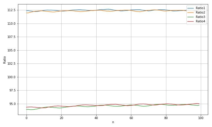
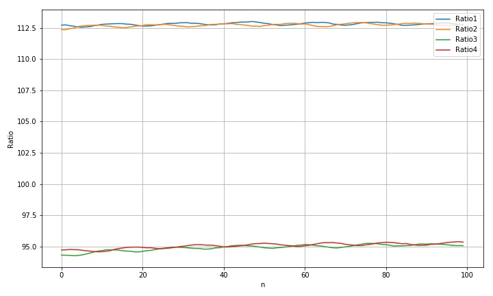
2.1.5 radius obtained by vertical movement
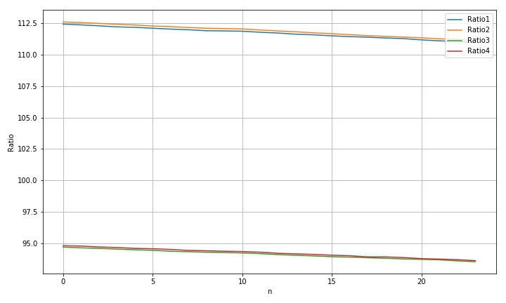
std(rdim1): 0.42990733097629413
std(rdim2): 0.44317522551733896
std(rdim3): 0.3398756613002497
std(rdim4): 0.35404918503322796
max(rdim1)-min(rdim1): 1.482045089816367
max(rdim2)-min(rdim2): 1.4698391609185535
max(rdim3)-min(rdim3): 1.1608641856747255
max(rdim4)-min(rdim4): 1.188417000120964
according to Scanner standard template sliding acquisition image and its processing Given the motion parameters, move 100 steps and the moving distance is about 20mm. Therefore, in the above movement of about 20 steps, the corresponding rising distance is 4mm, the pixel change of radius is 1.25 pixels, and the pixel change corresponding to 150dpi is 0.625. For the actual size, it is 0.11mm. Therefore, for every 1mm movement, the corresponding actual radius change is: 0.0265; The diameter changes by about 0.05.
※ test summary ※
using the area of the ring to calculate the radius of the circle in reverse, we can obtain a more stable radius of the circle. For the movement of the standard template on the scanner, you can see the change law of the corresponding measurement results. The following is a preliminary analysis of such changes.
- Moving along the transverse direction, we can see that the radius variation laws of the four circles are different, which may be due to the interference of the background light;
- Fluctuations in a circle moving diagonally. It is speculated that this may be due to the influence of the brightness change of the edge of the metal template caused by the fill light source corresponding to the scanner;
- The reason for the decrease of circle radius caused by the vertical rise of formwork is relatively clear. It can be calculated from the data that the diameter measurement result will be reduced by 0.05mm for every 1mm change in height.
3.1 remaining problems
the following problems remain:
1. The proportional change coefficient of the measurement results with the change of height is obtained above. We need to find some ways to compensate.
2. For the fluctuation caused by vertical and horizontal Yingdong, it is necessary to further find the reason through experiments and give the correction method.
■ links to relevant literature:
- Bacteriostatic circle
- Get pictures of different positions of checkerboard and standard template on the scanner
- Scanner standard template sliding acquisition image and its processing
● links to relevant charts:
- Figure 1.1.1 using a scanner to obtain the ring diameter in a metal circular template
- Figure 1.1.1 arrangement sequence of four rings
- Figure 1.1.2 position of pre extracted circle in horizontal scanning picture
- Figure 1.1.3 diagonal translation scanning picture
- Figure 1.1.4 picture of circle moving vertically
- Figure 2.1 circles after segmentation
- Figure 2.1.1 pixel brightness statistics converted to grayscale image
- Figure 2.1.2 find the outline in the black-and-white picture
- Fig. 2.1.3 change of radius of four rings with movement
- Figure 2.1.4 equivalent radius corresponding to the movement of four rings
- Figure 2.1.5 results of horizontal translation processing circle radius
- Figure 2.1.6 circle radius corresponding to vertical movement
#!/usr/local/bin/python
# -*- coding: gbk -*-
#============================================================
# TEST1.PY                     -- by Dr. ZhuoQing 2022-01-26
#
# Note:
#============================================================

from headm import *                 # =
import cv2
from tqdm import tqdm

#------------------------------------------------------------
#npzdiag = '/home/aistudio/work/Scanner/ScanDiagBlock.npz'
#scandiagdir = '/home/aistudio/work/Scanner/ScanDiagBlock'
#npzdiag = '/home/aistudio/work/Scanner/ScanRowBlock.npz'
#scandiagdir = '/home/aistudio/work/Scanner/ScanRowBlock'
npzdiag = '/home/aistudio/work/Scanner/ScanVertBlock.npz'
scandiagdir = '/home/aistudio/work/Scanner/ScanVertBlock'

filedim = sorted([s for s in os.listdir(scandiagdir) if s.find("jpg") > 0])
#printt(filedim:)

alldata = load(npzdiag, allow_pickle=True)
#printt(alldata.files:)
alldim = alldata['alldim']
allfile = alldata['allfile']

#printt(alldim:, allfile:)

#------------------------------------------------------------
block_side = 140
def img2block(img, circles):
    block = []
    for c in circles:
        left = int(c[0] - block_side)
        right = left + block_side*2
        top = int(c[1] - block_side)
        bottom = top + block_side*2

        block.append(img[top:bottom, left:right, :])

    return block

#------------------------------------------------------------
rdim1 = []
rdim2 = []
rdim3 = []
rdim4 = []

threshold = 100

for id,f in tqdm(enumerate(allfile)):
    img = cv2.imread(f)
    cc = alldim[id]

    if id >= 41: break

    #--------------------------------------------------------
'''
    for c in cc:
        printt(c:)
        cv2.circle(img, (c[0], c[1]), int(c[2]), (0,0,255), 10)

    plt.figure(figsize=(10,10))
    plt.imshow(img[:,:,::-1])

    break
'''
    #--------------------------------------------------------

    block = img2block(img, cc)

    #--------------------------------------------------------
'''
    plt.figure(figsize=(10,10))
    plt.subplot(2,2,1)
    plt.imshow(block[0])
    plt.subplot(2,2,2)
    plt.imshow(block[1])
    plt.subplot(2,2,3)
    plt.imshow(block[2])
    plt.subplot(2,2,4)
    plt.imshow(block[3])

    plt.savefig('/home/aistudio/stdout.jpg')
    break
'''
    #--------------------------------------------------------

#    plt.figure(figsize=(10,10))

    ratioDim = []
    for iidd,b in enumerate(block):
        bgray = cv2.cvtColor(b, cv2.COLOR_BGR2GRAY)
        threshold = mean(bgray.flatten())
        ret,thresh = cv2.threshold(bgray, threshold, 255, 0)
        contours,hierarchy = cv2.findContours(thresh, cv2.RETR_TREE, cv2.CHAIN_APPROX_NONE)
        cv2.drawContours(b, contours, -1, (0, 0, 255), 3)


        areaDim = []
        for id,c in enumerate(contours):
            areaDim.append(cv2.contourArea(c))

        asorted = sorted(areaDim)
        a = asorted[-2]
        r = sqrt(a/pi)
        ratioDim.append(r)


#        plt.subplot(2,2,iidd+1)
#        plt.hist(bgray.flatten(), bins=20)
#        plt.imshow(b[:,:,::-1])

#    printt(ratioDim:)
    if len(ratioDim) != 4: break

    rdim1.append(ratioDim[0])
    rdim2.append(ratioDim[1])
    rdim3.append(ratioDim[2])
    rdim4.append(ratioDim[3])

#    plt.savefig('/home/aistudio/stdout.jpg')
#    plt.show()


#    break


#------------------------------------------------------------
plt.clf()
plt.figure(figsize=(10,6))
plt.plot(rdim1, label='Ratio1')
plt.plot(rdim2, label='Ratio2')
plt.plot(rdim3, label='Ratio3')
plt.plot(rdim4, label='Ratio4')
plt.legend(loc="upper right")
plt.xlabel("n")
plt.ylabel("Ratio")
plt.grid(True)
plt.tight_layout()
plt.savefig('/home/aistudio/stdout.jpg')
plt.show()


#------------------------------------------------------------
printt(std(rdim1):,std(rdim2):,std(rdim3):,std(rdim4):)
printt(max(rdim1)-min(rdim1):)
printt(max(rdim2)-min(rdim2):)
printt(max(rdim3)-min(rdim3):)
printt(max(rdim4)-min(rdim4):)

#------------------------------------------------------------
#        END OF FILE : TEST1.PY
#============================================================