abstract
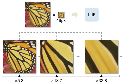
The physical world presents visual images in a continuous manner, but computers store and display images in the form of discrete 2D pixel arrays. This paper studies the continuous representation of the image, uses the Local Implicit Image Function (LIIF) to take the image coordinates and the 2D depth features around the coordinates as the input, and predicts the RGB value under the given coordinates. Through the self supervised super-resolution task to train an encoder and LIIF representation to generate the continuous representation of pixel image, the resolution of any multiple can be achieved, and even the super score of more than 30 times that is not in the training task can be calculated. By modeling the image as a function in the continuous domain, the image with arbitrary resolution can be restored and generated. The idea of implicit function is to represent an object as a function and map the coordinates to the corresponding signals (such as the symbol distance on the surface of 3D object and the RGB value in the image). The neural implicit function is parameterized by deep neural network. In order to share knowledge across instances instead of fitting a separate implicit function for each object, an encoder based method is proposed to predict the potential coding of each object. The implicit function is then shared by all objects, while it takes the underlying code as additional input.
Local Implicit Image Function
In the LIIF representation, each continuous image I ( i ) I^{(i)} I(i) is mapped by two-dimensional features M ( i ) ∈ R H × W × D M^{(i)}∈\R^{H \times W \times D} M(i)∈RH × W × D means. A neural implicit function f θ f_θ f θ (with) θ θ θ Is shared by all images, and it is parameterized as M L P MLP MLP and take s = f ( z , x ) s = f(z,x) S = f (Z, x) (omitted simply) θ θ θ) Form, where z z z is a vector, x ∈ X x \in X X ∈ x is a two-dimensional coordinate in the continuous image domain, s ∈ S s \in S ∈ s is the predicted value (RGB).
For defined f f f. Each vector z z z can be regarded as a representation function f ( z , ⋅ ) : X → S f(z,·):X→S f(z,⋅):X→S. f ( z , ⋅ ) f(z,·) f(z, ⋅) can be regarded as a continuous image, that is, a function of mapping coordinates to RGB values. hypothesis M ( i ) M^{(i)} Of M(i) H × W H \times W H × W eigenvectors (called latent codes) are evenly distributed in I ( i ) I^{(i)} I(i) in the 2D space of the continuous image domain, and assign a 2D coordinate to each of them.
For images
I
(
i
)
I^{(i)}
I(i), coordinates
x
q
x_q
The RGB value at xq is defined as
I
(
i
)
(
x
q
)
=
f
(
z
∗
,
x
q
−
v
∗
)
I^{(i)}(x_q) = f(z^*,x_q-v^*)
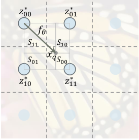
I(i)(xq) = f(z *, xq − v *), where
z
∗
z^∗
z * yes
M
(
i
)
M^{(i)}
In M(i) and
x
q
x_q
xq nearest (Euclidean distance) hidden code,
v
∗
v^∗
v * is the latent code in the image domain
z
∗
z^∗
Coordinates of z *. for example
z
11
∗
z^∗_{11}
z11 * is in the current definition
x
q
x_q
xq +
z
∗
z^∗
z *, and
v
∗
v^∗
v * is defined as
z
11
∗
z^∗_{11}
Coordinates of z11 *.
Implicit functions shared in all images
f
f
Under f, continuous images are mapped by two-dimensional features
M
(
i
)
∈
R
H
×
W
×
D
M^{(i)} \in \R^{H \times W \times D}
M(i)∈RH × W × D indicates that the feature map is considered to be evenly distributed in the 2D domain
H
×
W
H×W
H × W hidden code. stay
M
(
i
)
M^{(i)}
Each potential code in M(i)
z
z
z represents the local part of the continuous image, which is responsible for predicting the signal of its nearest coordinate set.
The normalized coordinate value and RGB value are obtained from the image
def make_coord(shape, ranges=None, flatten=True):
    """ Make coordinates at grid centers.
    """
    coord_seqs = []
    for i, n in enumerate(shape):
        if ranges is None:
            v0, v1 = -1, 1
        else:
            v0, v1 = ranges[i]
        r = (v1 - v0) / (2 * n)
        seq = v0 + r + (2 * r) * torch.arange(n).float()
        coord_seqs.append(seq)
    ret = torch.stack(torch.meshgrid(*coord_seqs), dim=-1)
    if flatten:
        ret = ret.view(-1, ret.shape[-1])
    return ret

coord = make_coord((h, w)) #h. W is the height and width of SR target

def to_pixel_samples(img):
    """ Convert the image to coord-RGB pairs.
        img: Tensor, (3, H, W)
    """
    coord = make_coord(img.shape[-2:])   #(h*w,2)--(h*w,[x,y])
    rgb = img.view(3, -1).permute(1, 0)  #(h*w,3)--(h*w,[R,G,B])
    return coord, rgb
Feature unfolding
In order to enrich the information contained in the hidden code, the feature
M
(
i
)
M^{(i)}
M(i) expansion
M
^
(
i
)
{\hat M^{(i)}}
M^(i).
M
^
(
i
)
{\hat M^{(i)}}
M^(i) is in
M
(
i
)
M^{(i)}
In M(i)
3
×
3
3 \times 3
three × 3. Merging of adjacent hidden codes.
M
^
j
k
(
i
)
=
C
o
n
c
a
t
(
{
M
j
+
l
,
k
+
m
(
i
)
}
l
,
m
∈
{
−
1
,
0
,
1
}
)
{\hat M^{(i)}_{jk}} =Concat(\{M^{(i)}_{j+l,k+m}\}_{l,m\in\{-1,0,1\}})
M^jk(i)=Concat({Mj+l,k+m(i)}l,m∈{−1,0,1})
When
C
o
n
c
a
t
Concat
Concat refers to the connection of a set of vectors,
M
(
i
)
M^{(i)}
M(i) is filled with a zero vector outside its boundary.
[
N
,
C
,
L
R
H
,
L
R
W
]
[N,C,LR_H,LR_W]
[N,C,LRH, LRW]
f
e
a
t
feat
feat is
u
n
f
o
l
d
unfold
unfold becomes
[
N
,
C
∗
3
∗
3
,
L
R
H
,
L
R
W
]
[N,C*3*3,LR_H,LR_W]
[N,C∗3∗3,LRH,LRW].
feat = F.unfold(feat, 3, padding=1).view(feat.shape[0], feat.shape[1] * 9, feat.shape[2], feat.shape[3])
Local ensemble
s
=
f
(
z
,
x
)
s = f(z,x)
s=f(z,x) is a discontinuous prediction because
x
q
x_q
xq signal prediction is through query
M
(
i
)
M^{(i)}
The nearest hidden code in M(i)
z
∗
z^∗
z * completed, so when
x
q
x_q
xq# when moving in the image domain,
z
∗
z^∗
z * will suddenly switch from one hidden code to another. stay
z
∗
z^∗
z * around those coordinates selected for switching, two signals infinitely close to the coordinates will be predicted from different implicit codes, as long as the learned implicit function
f
f
f is not perfect, in
z
∗
z^∗
z * there is no discontinuous figure at the boundary of the selected switch. In order to solve this problem, local integration technology is used to expand the representation of each hidden code
I
(
i
)
(
x
q
)
=
∑
t
∈
{
00
,
01
,
10
,
11
}
S
t
S
f
(
z
t
∗
,
x
q
−
v
t
∗
)
I^{(i)}(x_q) =\sum_{t\in\{00,01,10,11\}} \frac {S_t}{S} f(z^*_t,x_q-v^*_t)
I(i)(xq)=t∈{00,01,10,11}∑SStf(zt∗,xq−vt∗)
z
t
∗
(
t
∈
{
00
,
01
,
10
,
11
}
)
z^*_t(t\in\{00,01,10,11\})
zt * (t ∈ {00,01,10,11}) refers to the nearest hidden code in the upper left, upper right, lower left and lower right subspaces,
v
t
∗
v^*_t
vt * means
z
t
∗
z^*_t
The coordinates of zt *,
S
t
S_t
St # yes
x
q
x_q
xq # and
v
t
′
∗
v^*_{t'}
vt′∗(
v
t
′
∗
v^*_{t'}
vt '* yes
v
t
∗
v^*_{t}
The diagonal of vt *, such as the rectangular area between 00 to 11, 10 to 01). Weight by
S
=
∑
t
S
t
S=\sum_tS_t
S = ∑ t ∑ St normalization. Characteristic diagram
M
(
i
)
M^{(i)}
M(i) is mirror filled outside the boundary, so this also applies to the coordinates near the boundary.
This is to make the local image block represented by the hidden code overlap with its adjacent blocks, so that there are four hidden codes at each coordinate for the independent prediction signal. Then, the four predictions are combined by voting with normalized confidence, which is proportional to the rectangular area between the query point and its nearest diagonal corresponding point of the hidden code. Therefore, when the query coordinate is closer, the confidence becomes higher. By this vote, it z ∗ z^* The continuous transition is realized at the z * transformation coordinates (i.e. the dotted line in the figure).
vx_lst = [-1, 1]
vy_lst = [-1, 1]
eps_shift = 1e-6

rx = 2 / feat.shape[-2] / 2  #2/H/2
ry = 2 / feat.shape[-1] / 2  #2/W/2

feat_coord = make_coord(feat.shape[-2:], flatten=False).cuda() #[LR_H,LR_W,2]
feat_coord = feat_coord.permute(2, 0, 1).unsqueeze(0).expand(feat.shape[0], 2, *feat.shape[-2:])#[N,2,LR_H,LR_W]

preds = []
areas = []
for vx in vx_lst:
    for vy in vy_lst:
        coord_ = coord.clone()#[N,SR_H*SR_W,2]
        coord_[:, :, 0] += vx * rx + eps_shift
        coord_[:, :, 1] += vy * ry + eps_shift
        coord_.clamp_(-1 + 1e-6, 1 - 1e-6)

        q_feat = F.grid_sample(feat, coord_.flip(-1).unsqueeze(1),mode='nearest', align_corners=False)#[N,C*9,1,SR_H*SR_W]
        q_feat = q_feat[:, :, 0, :].permute(0, 2, 1)#[N,SR_H*SR_W,C*9]

        q_coord = F.grid_sample(feat_coord, coord_.flip(-1).unsqueeze(1),mode='nearest', align_corners=False)#[N,2,1,SR_H*SR_W]
        q_coord = q_coord[:, :, 0, :].permute(0, 2, 1)#[N,SR_H*SR_W,2]

        rel_coord = coord - q_coord #[N,SR_H*SR_W,2]
        rel_coord[:, :, 0] *= feat.shape[-2]
        rel_coord[:, :, 1] *= feat.shape[-1]
        inp = torch.cat([q_feat, rel_coord], dim=-1) #[N,SR_H*SR_W,C*9+2]

        if self.cell_decode:
            rel_cell = cell.clone()
            rel_cell[:, :, 0] *= feat.shape[-2]
            rel_cell[:, :, 1] *= feat.shape[-1]
            inp = torch.cat([inp, rel_cell], dim=-1) #[N,SR_H*SR_W,C*9+2+2]

        bs, q = coord.shape[:2] #bs=N q=SR_H*SR_W
        #[N*SR_H*SR_W,C*9+2+2] --> [N*SR_H*SR_W,3]
        pred = self.imnet(inp.view(bs * q, -1)).view(bs, q, -1) #[N,SR_H*SR_W,3]
        preds.append(pred) #[[N,SR_H*SR_W],[N,SR_H*SR_W],[N,SR_H*SR_W],[N,SR_H*SR_W]]

        area = torch.abs(rel_coord[:, :, 0] * rel_coord[:, :, 1])
        areas.append(area + 1e-9) #[[N,SR_H*SR_W],[N,SR_H*SR_W],[N,SR_H*SR_W],[N,SR_H*SR_W]]


tot_area = torch.stack(areas).sum(dim=0) #[N,SR_H*SR_W]
if self.local_ensemble:
    t = areas[0]; areas[0] = areas[3]; areas[3] = t #swap(areas[0],areas[3])
    t = areas[1]; areas[1] = areas[2]; areas[2] = t #swap(areas[1],areas[2])
Cell decoding
In order for LIIF to represent arbitrary resolution rendering based on pixel form, assuming the required resolution is given, a simple method is to query the continuous representation
I
(
∗
)
I^{(*)}
The RGB value at the center coordinate of the pixel in I(*), but because the predicted RGB value of the query pixel is independent of its size, the information in its pixel area except the center value is discarded, which may not be the best.
s
=
f
c
e
l
l
(
z
,
[
x
,
c
]
)
s=f_{cell}(z,[x,c])
s=fcell(z,[x,c])
c
=
[
c
h
,
c
w
]
c=[c_h,c_w]
c=[ch, cw] contains the height and width of the specified query pixel,
[
x
,
c
]
[x,c]
[x,c] is the value
x
x
x and
c
c
c connection,
c
c
c is additional input.
f
c
e
l
l
(
z
,
[
x
,
c
]
)
f_{cell}(z,[x,c])
fcell (z,[x,c]) can be understood as using shape
c
c
c render in coordinates
x
x
The RGB value of the pixel centered on x. about
64
×
64
64\times64
sixty-four × 64 resolution,
c
c
c is the width of the image
1
/
64
1/64
1/64. Logically, when
c
→
0
c→0
c → 0,
f
c
e
l
l
(
z
,
x
)
=
f
c
e
l
l
(
z
,
[
x
,
c
]
)
f_{cell}(z,x) =f_{cell}(z,[x,c])
Fcell (z,x)=fcell (z,[x,c]), that is, continuous images can be regarded as images with infinitely small pixels.
cell = torch.ones_like(coord) #[SR_H*SR_W,2] [1*2/SR_H,1*2/SR_W]
cell[:, 0] *= 2 / h
cell[:, 1] *= 2 / w

if self.cell_decode:
     rel_cell = cell.clone()
     rel_cell[:, :, 0] *= feat.shape[-2]
     rel_cell[:, :, 1] *= feat.shape[-1]
     inp = torch.cat([inp, rel_cell], dim=-1) #[N,SR_H*SR_W,C*9+2+2]
LIIF class full code
class LIIF(nn.Module):
    def __init__(self, encoder_spec, imnet_spec=None,
                 local_ensemble=True, feat_unfold=True, cell_decode=True):
        super().__init__()
        self.local_ensemble = local_ensemble
        self.feat_unfold = feat_unfold
        self.cell_decode = cell_decode
        self.encoder = models.make(encoder_spec)

        #print("self.encoder.out_dim",self.encoder.out_dim)
        if imnet_spec is not None:
            imnet_in_dim = self.encoder.out_dim     #64
            if self.feat_unfold:
                imnet_in_dim *= 9
            imnet_in_dim += 2 # Attach coach specifies the coordinates of the query pixel [x,y]
            if self.cell_decode:
                imnet_in_dim += 2 #[Cell_h, Cell_w] specify two values for the height and width of the query pixel
            self.imnet = models.make(imnet_spec, args={'in_dim': imnet_in_dim})
        else:
            self.imnet = None

    def gen_feat(self, inp):
        self.feat = self.encoder(inp)
        return self.feat

    def query_rgb(self, coord, cell=None):
        #coord [N,SR_H*SR_*W,2]
        #cell [N,SR_H*SR_*W,2]
        feat = self.feat #[N,C,LR_H,LR_W]

        if self.imnet is None:
            ret = F.grid_sample(feat, coord.flip(-1).unsqueeze(1), mode='nearest', align_corners=False)
            ret = ret[:, :, 0, :].permute(0, 2, 1)
            return ret

        if self.feat_unfold:
            # [N,C*3*3,H,W]
            feat = F.unfold(feat, 3, padding=1).view(feat.shape[0], feat.shape[1] * 9, feat.shape[2], feat.shape[3])

        if self.local_ensemble:
            vx_lst = [-1, 1]
            vy_lst = [-1, 1]
            eps_shift = 1e-6
        else:
            vx_lst, vy_lst, eps_shift = [0], [0], 0

        # field radius (global: [-1, 1])
        rx = 2 / feat.shape[-2] / 2  #2/H/2
        ry = 2 / feat.shape[-1] / 2  #2/W/2

        feat_coord = make_coord(feat.shape[-2:], flatten=False).cuda() #[LR_H,LR_W,2]
        feat_coord = feat_coord.permute(2, 0, 1).unsqueeze(0).expand(feat.shape[0], 2, *feat.shape[-2:])#[N,2,LR_H,LR_W]

        preds = []
        areas = []
        for vx in vx_lst:
            for vy in vy_lst:
                coord_ = coord.clone()#[N,SR_H*SR_W,2]
                coord_[:, :, 0] += vx * rx + eps_shift
                coord_[:, :, 1] += vy * ry + eps_shift
                coord_.clamp_(-1 + 1e-6, 1 - 1e-6)

                q_feat = F.grid_sample(feat, coord_.flip(-1).unsqueeze(1),mode='nearest', align_corners=False)#[N,C*9,1,SR_H*SR_W]
                q_feat = q_feat[:, :, 0, :].permute(0, 2, 1)#[N,SR_H*SR_W,C*9]

                q_coord = F.grid_sample(feat_coord, coord_.flip(-1).unsqueeze(1),mode='nearest', align_corners=False)#[N,2,1,SR_H*SR_W]
                q_coord = q_coord[:, :, 0, :].permute(0, 2, 1)#[N,SR_H*SR_W,2]

                rel_coord = coord - q_coord #[N,SR_H*SR_W,2]
                rel_coord[:, :, 0] *= feat.shape[-2]
                rel_coord[:, :, 1] *= feat.shape[-1]
                inp = torch.cat([q_feat, rel_coord], dim=-1) #[N,SR_H*SR_W,C*9+2]

                if self.cell_decode:
                    rel_cell = cell.clone()
                    rel_cell[:, :, 0] *= feat.shape[-2]
                    rel_cell[:, :, 1] *= feat.shape[-1]
                    inp = torch.cat([inp, rel_cell], dim=-1) #[N,SR_H*SR_W,C*9+2+2]

                bs, q = coord.shape[:2] #bs=N q=SR_H*SR_W
                #[N*SR_H*SR_W,C*9+2+2] --> [N*SR_H*SR_W,3]
                pred = self.imnet(inp.view(bs * q, -1)).view(bs, q, -1) #[N,SR_H*SR_W,3]
                preds.append(pred) #[[N,SR_H*SR_W],[N,SR_H*SR_W],[N,SR_H*SR_W],[N,SR_H*SR_W]]

                area = torch.abs(rel_coord[:, :, 0] * rel_coord[:, :, 1])
                areas.append(area + 1e-9) #[[N,SR_H*SR_W],[N,SR_H*SR_W],[N,SR_H*SR_W],[N,SR_H*SR_W]]


        tot_area = torch.stack(areas).sum(dim=0) #[N,SR_H*SR_W]
        if self.local_ensemble:
            t = areas[0]; areas[0] = areas[3]; areas[3] = t #swap(areas[0],areas[3])
            t = areas[1]; areas[1] = areas[2]; areas[2] = t #swap(areas[1],areas[2])
        ret = 0
        for pred, area in zip(preds, areas):
            ret = ret + pred * (area / tot_area).unsqueeze(-1)
        return ret

    def forward(self, inp, coord, cell):
        self.gen_feat(inp)
        return self.query_rgb(coord, cell)