RFM model is an important tool and means of Hengxing's customer value and profitability.Describe a customer's value by three indicators: his recent purchasing behavior, the overall frequency of purchases, and how much he spent.
< R: Last consumption time (interval from last consumption to reference time)
F: Frequency of consumption
# M: Amount consumed (total consumption amount)

Data cleaning

data format

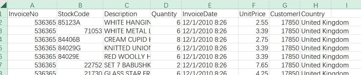
• InvoiceNo: Order number, 6 integers per transaction, return order number begins with the letter'C'.
• StockCode: The product number, which consists of five integers.
• Description: Product description.
• Quantity: Number of products, minus sign means return
• InvoiceDate: Order date and time.
• UnitPrice: Price per unit (pound sterling), price per unit product.
• CustomerID: Customer number. Each customer number consists of five digits.
• Country: Name of country, name of country/region where each customer is located.

df.shape

(541909, 8)

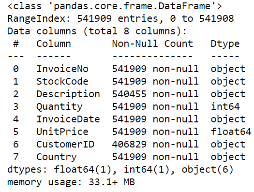
df.info()

Missing Statistics Rate

df.apply(lambda x:sum(x.isnull())/len(x),axis=0)

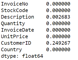
Item descriptions don't do much to directly delete this column, then delete rows with missing user IDs

df.drop(['Description'],axis=1,inplace=True)
# how	{‘Any','all'}, default'any', any: delete lines with nan;All: delete all NANs rows
df = df.dropna(how='any')

Data Standardization

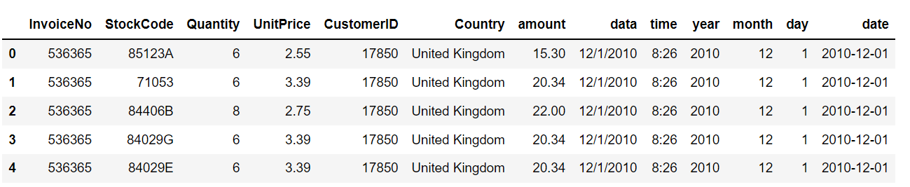
#Increase Total Purchase Amount = Quantity * Amount
df['amount']= df['Quantity']*df['UnitPrice']
#Order date slicing
df['data']=[x.split(' ')[0] for x in df['InvoiceDate']]
df['time']=[x.split(' ')[1] for x in df['InvoiceDate']]
df.drop(['InvoiceDate'],axis=1,inplace=True)
df['year']=[x.split('/')[2] for x in df['data']]
df['month']=[x.split('/')[0] for x in df['data']]
df['day']=[x.split('/')[1] for x in df['data']]
#Convert date format
df['date'] = pd.to_datetime(df['data'])
df.head()

Delete duplicate data

df = df.drop_duplicates()

Observe if there are outliers

df.describe()

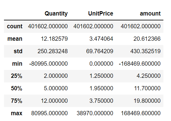
There are returned orders and items with a price of 0 (possibly gifts)
Return order percentage

df1 = df.loc[df['Quantity'] <= 0]
print(df1.shape[0]/df.shape[0])

0.022091523448588404

Price is 0 commodity ratio

df2 = df.loc[df['UnitPrice'] <= 0]
print(df2.shape[0]/df.shape[0])

0.0000996010976040956

Price is 0 number of items

df2['UnitPrice'].groupby(df2['UnitPrice']).count()

UnitPrice
0.0 40
Name: UnitPrice, dtype: int64

Calculate Return Rate
Number of returns/total orders

t_num = df1['Quantity'].sum()
sale_num = df[df['Quantity']>0]['Quantity'].sum()
t_rate = abs(t_num/sale_num)
print(t_rate)

0.05285657011028571

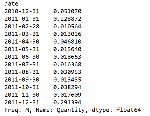
Monthly return rate

tt = df1.groupby(df1['date'])['Quantity'].sum()
tt = tt.resample('M').sum()
sale = df[df['Quantity']>0].groupby(df['date'])['Quantity'].sum()
sale = sale.resample('M').sum()
rate = abs(tt/sale)

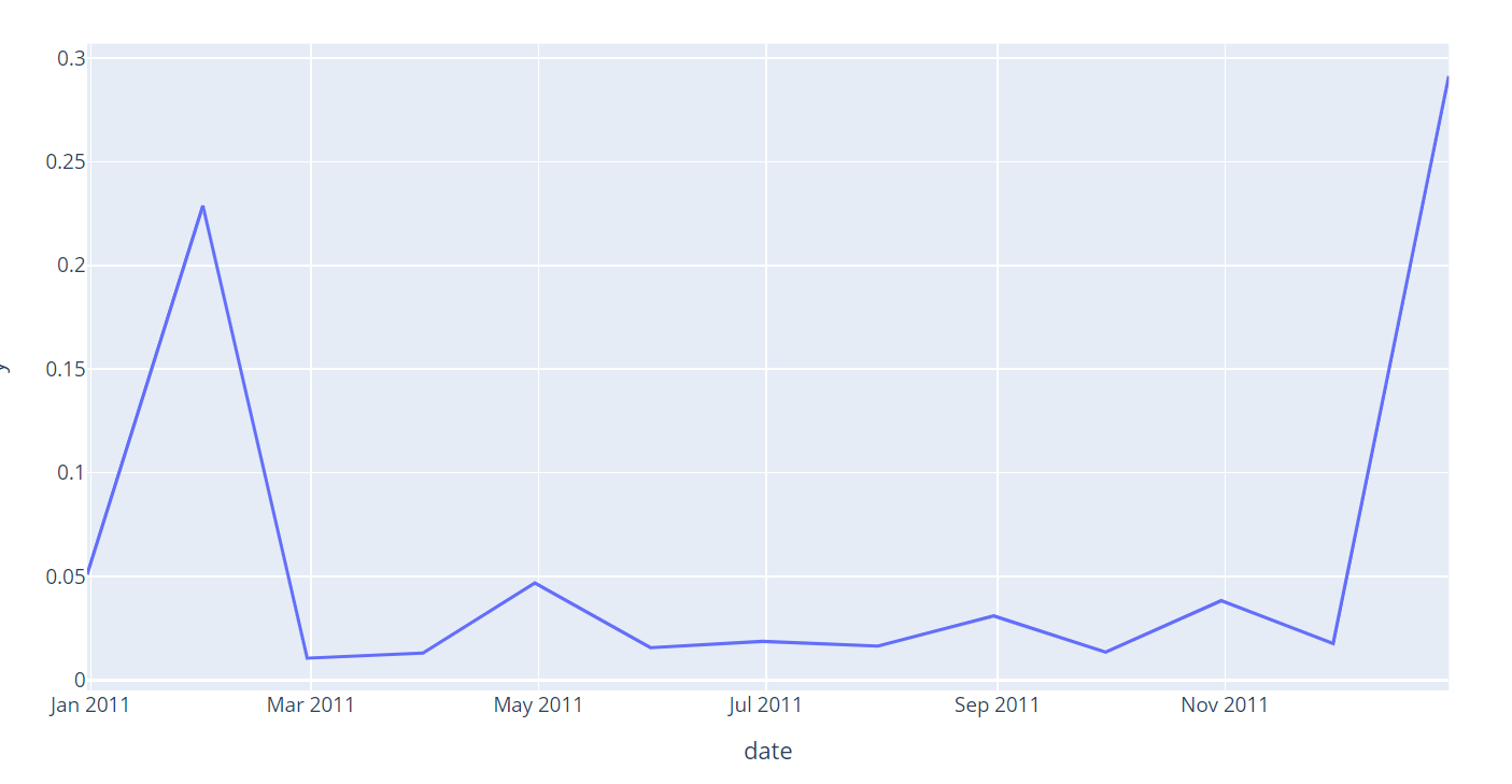
visualization

import plotly.express as px

_y = rate.values
_x = rate.index
fig = px.line(rate, x=_x, y=_y)
fig.show()

User Classification

df2 = df[(df['Quantity'] > 0)&(df['UnitPrice'] > 0)]
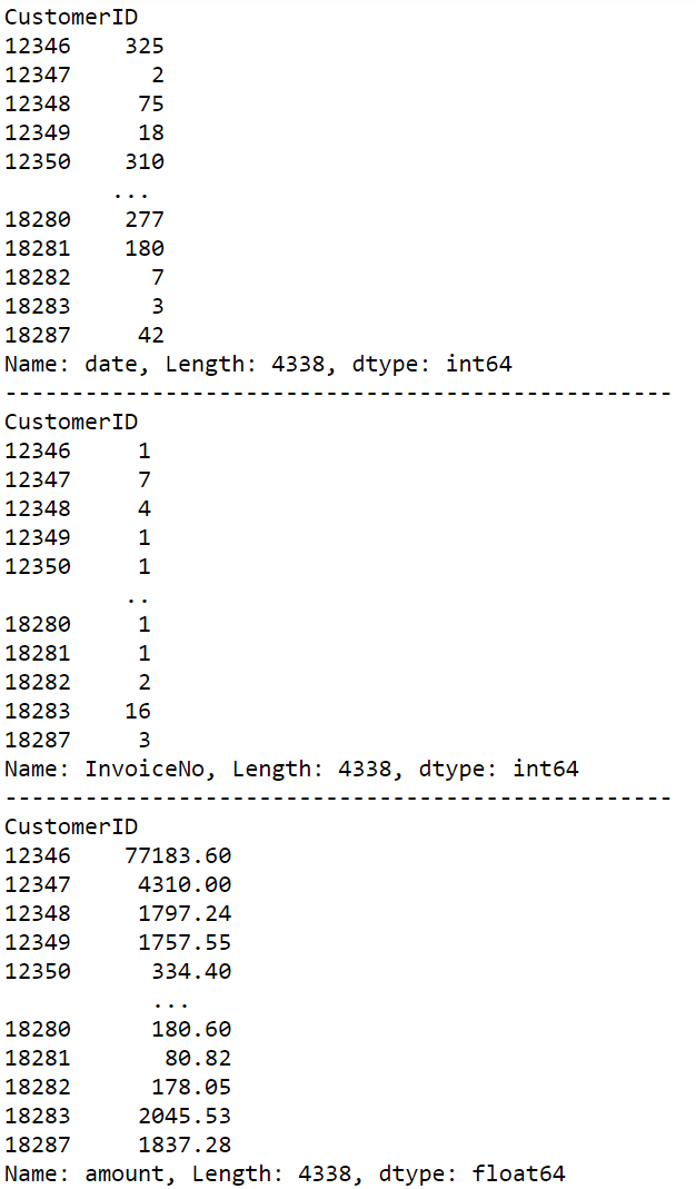
# Date of latest purchase
R_value=df2.groupby('CustomerID')['date'].max()
# Calculate customer's last consumption distance in days to deadline
R = (df2['date'].max()- R_value).dt.days
print(R)
print('-'*50)
#Customer consumption frequency, nunique:Number of calculations after weight removal
F = df2.groupby('CustomerID')['InvoiceNo'].nunique()
print(F)
print('-'*50)
#Customer consumption amount
M = df2.groupby('CustomerID')['amount'].sum()
print(M)

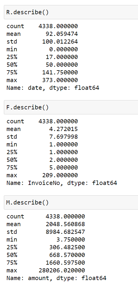
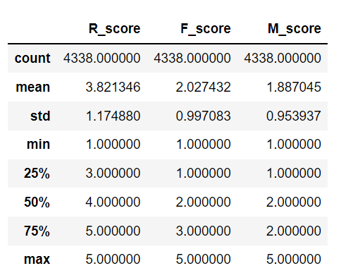
Find thresholds using describe() method

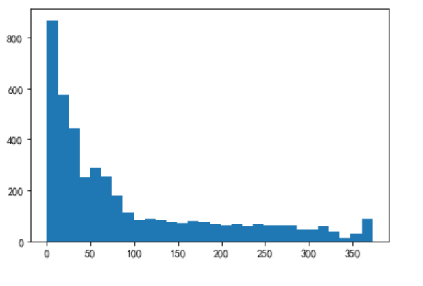
visualization
Visually display the distribution of data

plt.rcParams['font.sans-serif'] = ['SimHei']
plt.rcParams['axes.unicode_minus'] = False
plt.hist(R,bins =30) 
plt.show()

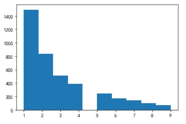
plt.hist(F,bins =30)
plt.show()

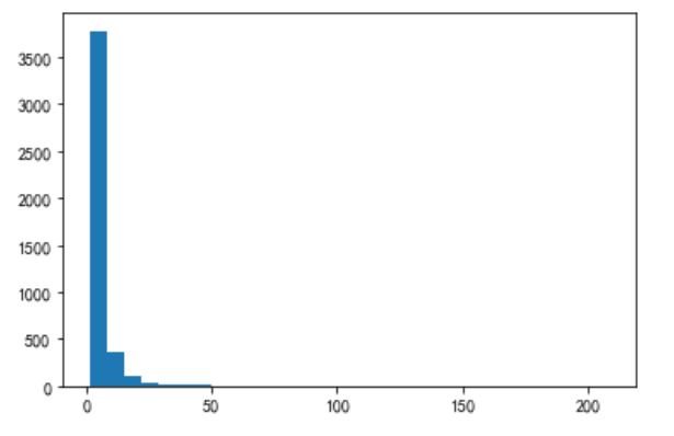
Visualization is not obvious affected by extreme values, observed within 10 days

print(F[F<10].count()/F.count())
plt.hist(F[F<10],bins =10)
plt.show

0.9098662978331028

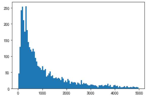
plt.hist(M,bins =30) 
plt.show

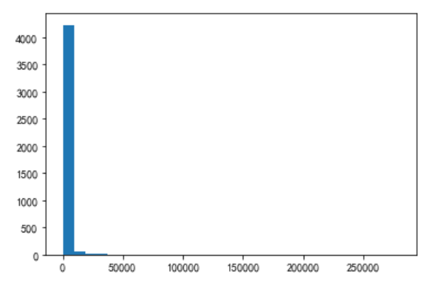
print(M[M<5000].count()/M.count())
plt.hist(M[M<5000],bins=100)
plt.show()

0.9368372521899493

Calculate rfm score

pd.cut() Inter-Zonal Statistics
Divide the data according to the above RFM distribution

R_bins = [0,30,90,180,360,720]  #Smaller is better
F_bins = [1,2,5,10,20,500]  #Larger is better
M_bins = [0,500,2000,5000,10000,300000] #Larger is better

R_score = pd.cut(R,R_bins, labels = [5,4,3,2,1], right=False)
F_score = pd.cut(F,F_bins, labels = [1,2,3,4,5], right=False)
M_score = pd.cut(M,M_bins, labels = [1,2,3,4,5], right=False)

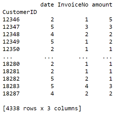
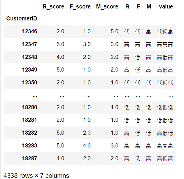
Data consolidation

rfm = pd.concat([R_score,F_score,M_score],axis=1)
print(rfm)

rfm.rename(columns={'date':'R_score','InvoiceNo':'F_score','amount':'M_score'},inplace = True)

Data Type Conversion

for i in ['R_score','F_score','M_score']:
    rfm[i] = rfm[i].astype(float)

View RFM Score Information

rfm.describe()

Ranking

rfm['R'] = np.where(rfm['R_score']>3.82,'high','low')
rfm['F'] = np.where(rfm['F_score']>2.03,'high','low')
rfm['M'] = np.where(rfm['M_score']>1.89,'high','low')
rfm['value'] = rfm['R'].str[:] + rfm['F'].str[:]+rfm['M'].str[:]
# Remove whitespace
rfm['value'] = rfm['value'].str.strip()

def trans_value(x):
    if x=='High and High':
        return 'Important Value Customer'
    elif x =='High and low':
        return 'Important Customer Development'
    elif x =='Low High':
        return 'Important customer retention'
    elif x =='Low Low High':
        return 'Important customer retention'
    elif x == 'High or low':
        return 'General Value Customer'
    elif x =='High or low':
        return 'General Customer Development'
    elif x =='Low or low':
        return 'Maintain customer in general'
    else:
        return 'Customer retention in general'

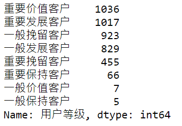
rfm['User Level'] = rfm['value'].apply(trans_value)
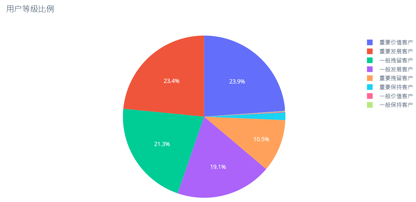
rfm['User Level'].value_counts()

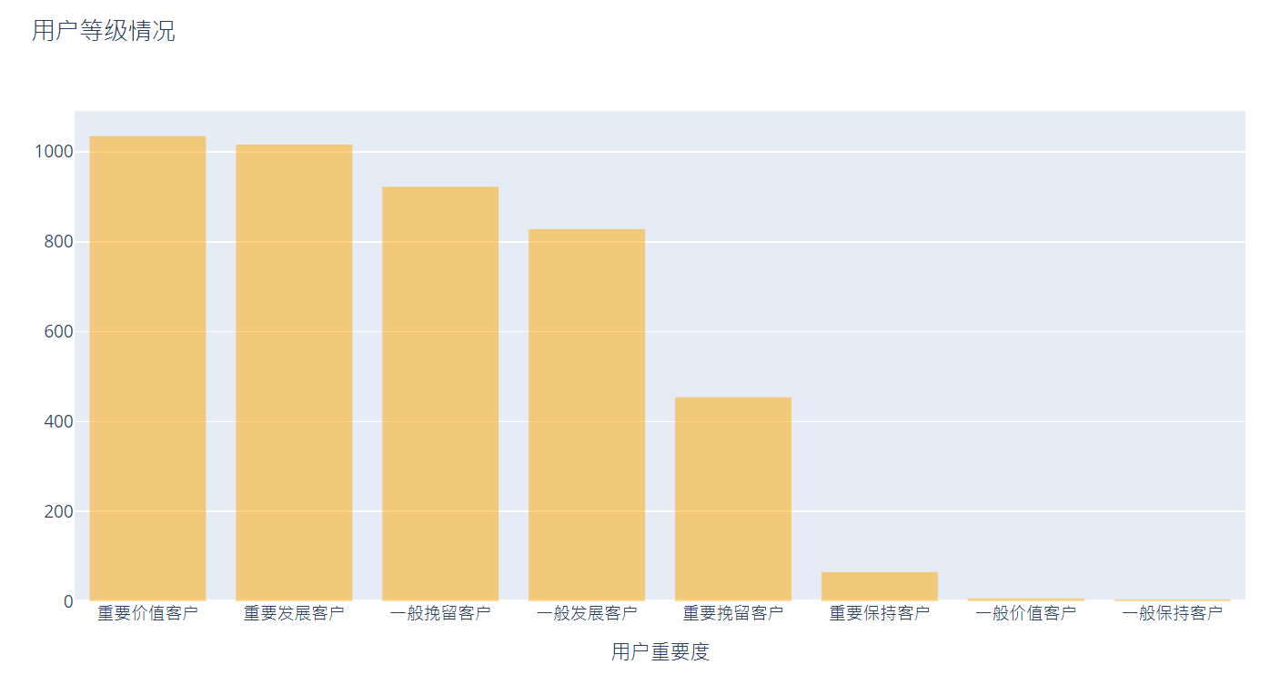
Visualize user level

trace_basic = [go.Bar(x =rfm['User Level'].value_counts().index.tolist(),
                      y =rfm['User Level'].value_counts().values.tolist(),
                      marker=dict(color='orange'),opacity=0.50)] #transparency
layout = go.Layout(title = 'User ratings',xaxis =dict(title ='User Importance'))
figure_basic = go.Figure(data = trace_basic,layout=layout)# data and layout form an image object
pyplot(figure_basic)

trace = [go.Pie(labels = rfm['User Level'].value_counts().index,values=rfm['User Level'].value_counts().values,
                textfont =dict(size=12,color ='white'))]
layout = go.Layout(title ='User Rating Scale')
fig = go.Figure(data = trace,layout=layout)
pyplot(fig)