1.MATLAB program implementation
The code is as follows:
%% Clear environment variables
clear;
clc;
close all;
%% Initialization parameters
data = rand(400, 2);
figure;
plot(data(:, 1), data(:, 2), 'ro', 'MarkerSize', 8);
xlabel 'Abscissa X'; ylabel 'Ordinate';
title 'sample data ';
K = 4; % Number of classifications
maxgen = 100; % Maximum number of iterations
alpha = 3; % Power of exponent
threshold = 1e-6; % threshold
[data_n, in_n] = size(data); % Number of rows, i.e. number of samples/Number of columns, i.e. sample dimension
% Initialize membership matrix
U = rand(K, data_n);
col_sum = sum(U);
U = U./col_sum(ones(K, 1), :);
%% iteration
for i = 1:maxgen
% Update cluster center
mf = U.^alpha;
center = mf*data./((ones(in_n, 1)*sum(mf'))');
% Update objective function value
dist = zeros(size(center, 1), data_n);
for k = 1:size(center, 1)
dist(k, :) = sqrt(sum(((data-ones(data_n, 1)*center(k, :)).^2)', 1));
end
J(i) = sum(sum((dist.^2).*mf));
% Update membership matrix
tmp = dist.^(-2/(alpha-1));
U = tmp./(ones(K, 1)*sum(tmp));
% Judgment of termination conditions
if i > 1
if abs(J(i) - J(i-1)) < threshold
break;
end
end
end
%% mapping
[max_vluae, index] = max(U);
index = index';
figure;
for i = 1:K
col = find(index == i); % max(U)Return the row where the maximum value of the membership column is consistent, which is divided into one category
plot(data(col, 1), data(col, 2), '*', 'MarkerSize', 8);
hold on
end
grid on
% Draw the cluster center
plot(center(:, 1), center(:, 2), 'p', 'color', 'm', 'MarkerSize', 12);
xlabel 'Abscissa X'; ylabel 'Ordinate Y';
title 'FCM Optimized clustering graph';
% Objective function change process
figure;
plot(J, 'r', 'linewidth', 2);
xlabel 'Number of iterations'; ylabel 'Objective function value';
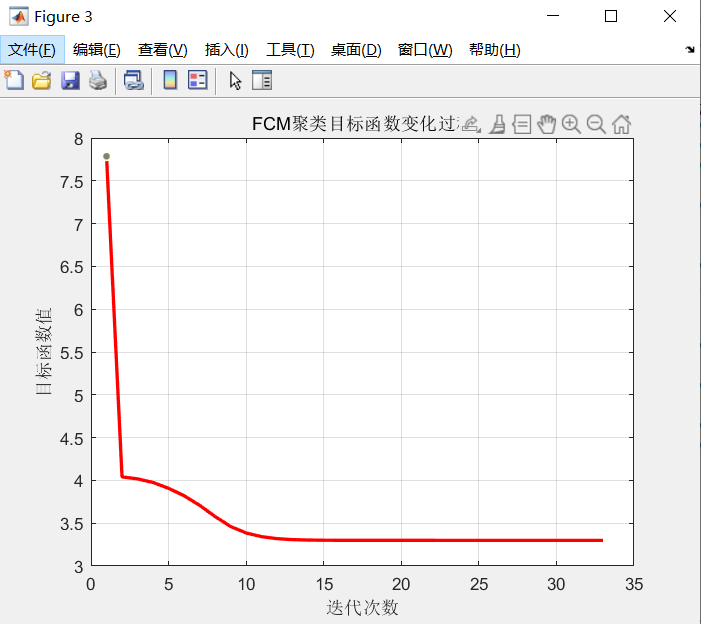
title 'FCM Change process of clustering objective function';
grid on
The clustering diagram after FCM optimization is shown in the figure
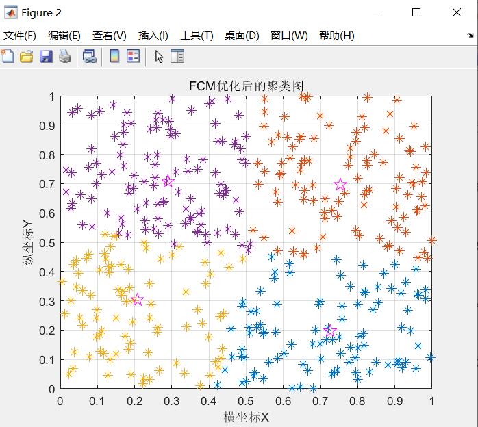 Successful clustering
The change process of FCM clustering objective function value is shown in the figure
2. Image segmentation based on fcm
A small example
The code is as follows:
clc
clear
close all
img = double(imread('lena.jpg'));
subplot(1,2,1),imshow(img,[]);
data = img(:);
%Divided into 4 categories
[center,U,obj_fcn] = fcm(data,4);
[~,label] = max(U); %Find the class to which you belong
%Change to image size
img_new = reshape(label,size(img));
subplot(1,2,2),imshow(img_new,[]);
You need to download the pictures yourself and go to the MATLAB directory
2. Image segmentation based on fcm
Data source website
http://archive.ics.uci.edu/ml/datasets/seeds#
This database is about seed classification. It contains three types of seeds and collects their characteristics. Each seed has seven eigenvalues to represent it (that is, it is equivalent to seven dimensions in the data). Each type of seed has 70 samples, so the whole data set is a 210 * 7 sample set. Download the sample set of matlab as txt file and save it in the directory above
The code is as follows:
clc
clear
close all
data = importdata('data.txt');
%data There is also column 8, the correct label column
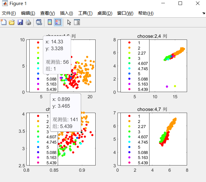
subplot(2,2,1);
gscatter(data(:,1),data(:,6),data(:,8)),title('choose:1,6 column')
subplot(2,2,2);
gscatter(data(:,2),data(:,4),data(:,8)),title('choose:2,4 column')
subplot(2,2,3);
gscatter(data(:,3),data(:,5),data(:,8)),title('choose:3,5 column')
subplot(2,2,4);
gscatter(data(:,4),data(:,7),data(:,8)),title('choose:4,7 column')
clc
clear
close all
data = importdata('seeds_dataset.txt');
%data There is also column 8, the correct label column
[center,U,obj_fcn] = fcm(data(:,1:7),3);
[~,label] = max(U); %Find the class to which you belong
subplot(1,2,1);
gscatter(data(:,4),data(:,7),data(:,8)),title('choose:4,7 column,Theoretical results')
% cal accuracy
a_1 = size(find(label(1:70)==1),2);
a_2 = size(find(label(1:70)==2),2);
a_3 = size(find(label(1:70)==3),2);
a = max([a_1,a_2,a_3]);
b_1 = size(find(label(71:140)==1),2);
b_2 = size(find(label(71:140)==2),2);
b_3 = size(find(label(71:140)==3),2);
b = max([b_1,b_2,b_3]);
c_1 = size(find(label(141:210)==1),2);
c_2 = size(find(label(141:210)==2),2);
c_3 = size(find(label(141:210)==3),2);
c = max([c_1,c_2,c_3]);
accuracy = (a+b+c)/210;
% plot answer
subplot(1,2,2);
gscatter(data(:,4),data(:,7),label),title(['Actual results,accuracy=',num2str(accuracy)])
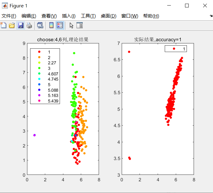
There's a problem. I came out with accuracy=1. According to the original author, it should not be able to achieve such accuracy
Comparison with Kmeans algorithm
1.1 data sources
The data comes from UCI database, which is a database for machine learning proposed by the University of California Irvine. UCI dataset is a commonly used standard test dataset.
website: http://archive.ics.uci.edu/ml/datasets/Solar+Flare
1.2 data description
Solar flare data set: each type of attribute counts the number of a certain type of flare in a 24-hour cycle solar flare data set
The code is as follows: FCM algorithm
m=1389;
n=13;
data=cell(m,n);%definition cell Matrix, storing file contents
fid=fopen('solar.txt','r');%Open file as read-only
for i=1:m
for j=1:n
data{i,j}=fscanf(fid,'%s',[1,1]);%Read each value in character mode, and complete the reading of each value in case of space
end
end
fclose (fid);
for i=1:m
for j=4:n
data{i,j}=str2double(data{i,j});%Convert text format to number format
end
end
str=cell(m,1); %For storage data Column 1 of
for i=1:m
str{i}=data{i,1};
end
str=cell(m,2); %For storage data Column 2 of
for i=1:m
str{i}=data{i,2};
end
str=cell(m,3); %For storage data Column 3 of
for i=1:m
str{i}=data{i,3};
end
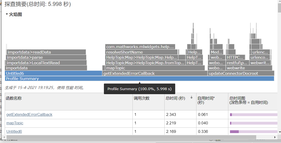
The code is as follows: Kmeans algorithm
m=1389;
n=13;
data=cell(m,n);%definition cell Matrix, storing file contents
fid=fopen('solar.txt','r');%Open file as read-only
for i=1:m
for j=1:n
data{i,j}=fscanf(fid,'%s',[1,1]);%Read each value in character mode, and complete the reading of each value in case of space
end
end
fclose (fid);
for i=1:m
for j=4:n
data{i,j}=str2double(data{i,j});%Convert text format to number format
end
end
str=cell(m,1); %For storage data Column 1 of
for i=1:m
str{i}=data{i,1};
end
str=cell(m,2); %For storage data Column 2 of
for i=1:m
str{i}=data{i,2};
end
str=cell(m,3); %For storage data Column 3 of
for i=1:m
str{i}=data{i,3};
end
Comparison of running time between two algorithms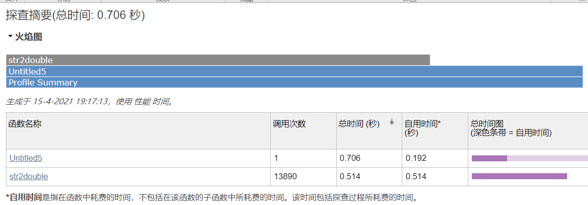
The clustering code of Kmeans is as follows:
% Number of cluster centers k
K = 3;
data  = importdata('flare1.txt');
x = data(:,1);
y = data(:,2);
% Drawing data, 2-D scatter diagram
% x,y: Data points to plot 20:The size of scatter points is the same, both of which are 20  'blue':The scatter color is blue
s = scatter(x, y, 20, 'blue');
title('Original data: blue circle; Initial cluster center: red dot');
% Initialize cluster center
sample_num = size(data, 1);       % Number of samples
sample_dimension = size(data, 2); % Characteristic dimension of each sample
% For the time being, manually specify the initial position of cluster center
% clusters = zeros(K, sample_dimension);
% Initial value of cluster center: calculate the mean value of all data, and add some small random vectors to the mean value
clusters = zeros(K, sample_dimension);
minVal = min(data); % Calculate the minimum value of each dimension
maxVal = max(data); % Calculate the maximum value of each dimension
for i=1:K
    clusters(i, :) = minVal + (maxVal - minVal) * rand();
end
hold on; % Prepare the next drawing based on the last drawing (scatter diagram)
% Draw initial cluster center
scatter(clusters(:,1), clusters(:,2), 'red', 'filled'); % A solid dot indicates the initial position of the cluster center
c = zeros(sample_num, 1); % The number of the cluster to which each sample belongs
PRECISION = 0.001;
iter = 100; % Assume a maximum of 100 iterations
% Stochastic Gradient Descendant Random gradient descent( SGD)of K-means,that is Competitive Learning edition
basic_eta = 1;  % learning rate
for i=1:iter
    pre_acc_err = 0;  % Cumulative error in the last iteration
    acc_err = 0;  % Cumulative error
    for j=1:sample_num
        x_j = data(j, :);     % Get the second j Sample data, which reflects stochastic nature
        % All cluster centers and x Calculate the distance and find the nearest one (compare the cluster center to x (mold length)
        gg = repmat(x_j, K, 1);
        gg = gg - clusters;
        tt = arrayfun(@(n) norm(gg(n,:)), (1:K)');
        [minVal, minIdx] = min(tt);
        % Update cluster center: update the nearest cluster center(winner)To data x Pull. eta Learning rate.
        eta = basic_eta/i;
        delta = eta*(x_j-clusters(minIdx,:));
        clusters(minIdx,:) = clusters(minIdx,:) + delta;
        acc_err = acc_err + norm(delta);
        c(j)=minIdx;
    end
    if(rem(i,10) ~= 0)
        continue
    end
    figure;
    f = scatter(x, y, 20, 'blue');
    hold on;
    scatter(clusters(:,1), clusters(:,2), 'filled'); % A solid dot indicates the initial position of the cluster center
    title(['The first', num2str(i), 'Second iteration']);
    if (abs(acc_err-pre_acc_err) < PRECISION)
        disp(['Converge to the second', num2str(i), 'Second iteration']);
        break;
    end
    disp(['Cumulative error:', num2str(abs(acc_err-pre_acc_err))]);
    pre_acc_err = acc_err;
end
disp('done');
reference
[1] Ding Zhen, Hu Zhongshan, Yang Jingyu, Tang Zhenmin, Wu Yongge An image segmentation method based on fuzzy clustering [J] Computer research and development, 1997 (07): 58-63
https://kns.cnki.net/kcms/detail/detail.aspx?dbcode=CJFD&dbname=CJFD9697&filename=JFYZ707.010&v=w6SVTbw2DI2U34NVEeHDiFy05S7tiJCXLSfhjzv1%25mmd2FMSAC%25mmd2B9EffWET8YmGo7%25mmd2BGjxA
[2] The principle and application of FCM algorithm CSDN
Link to this article: https://blog.csdn.net/on2way/article/details/47087201
[3] Implementation and comparative analysis of FCM clustering and K-means clustering CSDN
Link to this article: https://blog.csdn.net/weixin_45583603/article/details/102773689
[4] Clustering algorithm based on FCM algorithm CSDN
Link to this article: https://blog.csdn.net/weixin_43821559/article/details/113616617