1. Data operation
In PyTorch, torch Tensor is the main tool for storing and transforming data. If you have used NumPy before, you will find that tensor and NumPy's multidimensional arrays are very similar. However, tensor provides more functions such as GPU calculation and automatic gradient calculation, which makes tensor more suitable for deep learning.
The word "tensor" can generally be translated into "tensor", which can be regarded as a multi-dimensional array. Scalar can be regarded as 0-dimensional tensor, vector can be regarded as 1-dimensional tensor and matrix can be regarded as 2-dimensional tensor.
1.1 creating Tensor
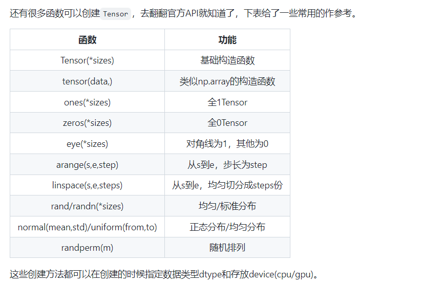
Let's first introduce the most basic function of Tensor, that is, the creation of Tensor.
Import PyTorch first:
import torch
Then we create a 5x3 uninitialized Tensor:
x = torch.empty(5, 3)
print(x)
Output:
tensor([[ 0.0000e+00,  1.5846e+29,  0.0000e+00],
        [ 1.5846e+29,  5.6052e-45,  0.0000e+00],
        [ 0.0000e+00,  0.0000e+00,  0.0000e+00],
        [ 0.0000e+00,  0.0000e+00,  0.0000e+00],
        [ 0.0000e+00,  1.5846e+29, -2.4336e+02]])
x = torch.tensor([1, 2])
x
tensor([1, 2])
Create a 5x3 randomly initialized Tensor:
x = torch.rand(5, 3)
print(x)
Output:
tensor([[0.4963, 0.7682, 0.0885],
        [0.1320, 0.3074, 0.6341],
        [0.4901, 0.8964, 0.4556],
        [0.6323, 0.3489, 0.4017],
        [0.0223, 0.1689, 0.2939]])
Create a 5x3 long all 0 Tensor:
x = torch.zeros(5, 3, dtype=torch.long)
print(x)
Output:
tensor([[0, 0, 0],
        [0, 0, 0],
        [0, 0, 0],
        [0, 0, 0],
        [0, 0, 0]])
You can also create directly from the data:
x = torch.tensor([5.5, 3])
print(x)
Output:
tensor([5.5000, 3.0000])
It can also be created through the existing Tensor. This method will reuse some properties of the input Tensor by default, such as data type, unless the data type is customized.
x = x.new_ones(5, 3, dtype=torch.float64)  # The returned tensor has the same torch by default Dtype and torch device
print(x)

x = torch.randn_like(x, dtype=torch.float) # Specify a new data type
print(x)
Output:
tensor([[1., 1., 1.],
        [1., 1., 1.],
        [1., 1., 1.],
        [1., 1., 1.],
        [1., 1., 1.]], dtype=torch.float64)
tensor([[ 0.6035,  0.8110, -0.0451],
        [ 0.8797,  1.0482, -0.0445],
        [-0.7229,  2.8663, -0.5655],
        [ 0.1604, -0.0254,  1.0739],
        [ 2.2628, -0.9175, -0.2251]])
We can get the shape of Tensor through shape or size():
print(x.size())
print(x.shape)
Output:
torch.Size([5, 3])
torch.Size([5, 3])
Note: the returned torch Size is actually a tuple, which supports all tuple operations.
1.2 operation (this section introduces various operations of Tensor)
(1) Arithmetic operation
In PyTorch, there may be many forms of the same operation. The following uses addition as an example.
- Additive form I
y = torch.rand(5, 3)
print(x + y)
- Additive form 2
print(torch.add(x, y))
You can also specify the output:
result = torch.empty(5, 3)
torch.add(x, y, out=result)
print(result)
- Additive form three inplace
# adds x to y
y.add_(x)
print(y)
Note: PyTorch operation inplace version has suffix, For example, x.copy_(y), x.t_ ()
Note: torch add_ () underlined here indicates that it is an in place function that will change the value of x
Generally speaking, functions underlined belong to built-in functions, which will change the original value. Functions not underlined will not change the original data. Additional values need to be assigned to other variables during reference
The output of the above forms are:
tensor([[ 1.3967,  1.0892,  0.4369],
        [ 1.6995,  2.0453,  0.6539],
        [-0.1553,  3.7016, -0.3599],
        [ 0.7536,  0.0870,  1.2274],
        [ 2.5046, -0.1913,  0.4760]])
(2) Index
We can also use an index operation similar to NumPy to access part of Tensor. It should be noted that the indexed results share memory with the original data, that is, if one is modified, the other will be modified.
y = x[0, :]
y += 1
print(y)
print(x[0, :]) # The source tensor has also been changed
Output:
tensor([1.6035, 1.8110, 0.9549])
tensor([1.6035, 1.8110, 0.9549])
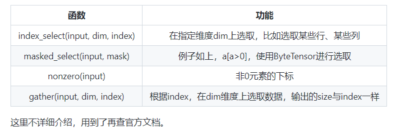
In addition to the commonly used index selection data, PyTorch also provides some advanced selection functions:
(3) Change shape (view, reshape, item)
Use view() to change the shape of Tensor:
y = x.view(15)
z = x.view(-1, 5)  # -1 refers to a dimension that can be derived from the values of other dimensions
print(x.size(), y.size(), z.size())
print(x)
print(y)
print(z)
Output:
torch.Size([5, 3]) torch.Size([15]) torch.Size([3, 5])

tensor([[-0.5807,  0.4220,  0.6563],
        [ 1.0477,  0.2788,  2.0502],
        [ 1.2781, -1.0631,  0.7602],
        [-1.0992,  0.1271, -0.7069],
        [-2.1188, -0.6162,  0.1537]])

tensor([-0.5807,  0.4220,  0.6563,  1.0477,  0.2788,  2.0502,  1.2781, -1.0631,
         0.7602, -1.0992,  0.1271, -0.7069, -2.1188, -0.6162,  0.1537])

tensor([[-0.5807,  0.4220,  0.6563,  1.0477,  0.2788],
        [ 2.0502,  1.2781, -1.0631,  0.7602, -1.0992],
        [ 0.1271, -0.7069, -2.1188, -0.6162,  0.1537]])
Note that the new Tensor returned by view() may have different size s from the source Tensor, but they share data, that is, changing one of them will change the other. (as the name suggests, view only changes the observation angle of this Tensor, and the internal data does not change)
x += 1
print(x)
print(y) # Also added 1
tensor([[ 0.4193,  1.4220,  1.6563],
        [ 2.0477,  1.2788,  3.0502],
        [ 2.2781, -0.0631,  1.7602],
        [-0.0992,  1.1271,  0.2931],
        [-1.1188,  0.3838,  1.1537]])
tensor([ 0.4193,  1.4220,  1.6563,  2.0477,  1.2788,  3.0502,  2.2781, -0.0631,
         1.7602, -0.0992,  1.1271,  0.2931, -1.1188,  0.3838,  1.1537])
So what if we want to return a really new copy (i.e. no shared data memory)? Pytorch also provides a * * reshape() * * function that can change the shape, but this function does not guarantee that it will return a copy, so it is not recommended. It is recommended to create a copy with clone first, and then use view. Refer here
Another advantage of using clone is that it will be recorded in the calculation diagram, that is, when the gradient is returned to the copy, it will also be transferred to the source Tensor.
x_cp = x.clone().view(15)
x -= 1
print(x)
print(x_cp)
tensor([[-0.5807,  0.4220,  0.6563],
        [ 1.0477,  0.2788,  2.0502],
        [ 1.2781, -1.0631,  0.7602],
        [-1.0992,  0.1271, -0.7069],
        [-2.1188, -0.6162,  0.1537]])
tensor([ 0.4193,  1.4220,  1.6563,  2.0477,  1.2788,  3.0502,  2.2781, -0.0631,
         1.7602, -0.0992,  1.1271,  0.2931, -1.1188,  0.3838,  1.1537])
Another common function is item(), which can convert a scalar Tensor into a Python number:
x = torch.randn(1)
print(x)
print(x.item())
tensor([2.3466])
2.3466382026672363
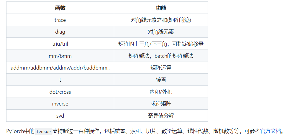
(3) Linear algebra
In addition, PyTorch also supports some linear functions, which are mentioned here to avoid making wheels by yourself when using them. Refer to the official documents for specific usage. As shown in the following table:
1.3 broadcasting mechanism
Previously, we saw how to perform element by element operation on two tensors with the same shape. When two tensors with different shapes are calculated by elements, the broadcasting mechanism may be triggered: first copy the elements appropriately to make the two tensors have the same shape, and then calculate by elements. For example:
x = torch.arange(1, 3).view(1, 2)
print(x)
y = torch.arange(1, 4).view(3, 1)
print(y)
print(x + y)
tensor([[1, 2]])
tensor([[1],
        [2],
        [3]])
tensor([[2, 3],
        [3, 4],
        [4, 5]])
Since X and y are matrices with one row, two columns and three rows and one column respectively, if x + y is to be calculated, the two elements of the first row in X are broadcast (copied) to the second row and the third row, while the three elements of the first column in y are broadcast (copied) to the second column. In this way, two matrices with three rows and two columns can be added by elements.
1.4 memory overhead of operation
As mentioned earlier, the index operation will not open up new memory, while operations such as y = x + y will open up new memory, and then point y to the new memory. To demonstrate this, we can use Python's own ID function: if the IDs of two instances are the same, their corresponding memory addresses are the same; Otherwise, it is different.
x = torch.tensor([1, 2])
y = torch.tensor([3, 4])
id_before = id(y)
y = y + x
print(id(y) == id_before) # False
If you want to specify the result to the memory of the original y, we can use the index described above to replace it. In the following example, we write the result of x + y into the memory corresponding to y through [:].
x = torch.tensor([1, 2])
y = torch.tensor([3, 4])
id_before = id(y)
y[:] = y + x
print(id(y) == id_before) # True
We can also use the out parameter in the operator full name function or the self addition operator + = (i.e. add_ ()) to achieve the above effect, such as torch Add (x, y, out = y) and y += x(y.add_(x)).
x = torch.tensor([1, 2])
y = torch.tensor([3, 4])
id_before = id(y)
torch.add(x, y, out=y) # y += x, y.add_(x)
print(id(y) == id_before) # True
Note: Although the Tensor returned by view shares data with the source Tensor, it is still a new Tensor (because Tensor has some other attributes bes id es data), and their IDs (memory addresses) are not consistent.
1.5 conversion between tensor and NumPy
It's easy to use NumPy () and from_numpy() converts arrays in Tensor and NumPy to each other. However, it should be noted that the arrays in Tensor and NumPy generated by these two functions share the same memory (so the conversion between them is fast). When changing one of them, the other will also change!!
Another common method to convert the array in NumPy into tensor is torch Tensor(), it should be noted that this method will always copy data (which will consume more time and space), so the returned tensor and the original data will no longer share memory.
(1)Tensor to NumPy
Convert Tensor to NumPy array using numpy():
a = torch.ones(5)
b = a.numpy()
print(a)
print(b)

a += 1
print(a)
print(b)

b += 1
print(a)
print(b)
tensor([1., 1., 1., 1., 1.])
[1. 1. 1. 1. 1.]

tensor([2., 2., 2., 2., 2.])
 [2. 2. 2. 2. 2.]

tensor([3., 3., 3., 3., 3.])
 [3. 3. 3. 3. 3.]
(2)NumPy array to Tensor
Use from_numpy() converts NumPy array to Tensor:
import numpy as np
a = np.ones(5)
b = torch.from_numpy(a)
print(a, b)

a += 1
print(a, b)
b += 1
print(a, b)
[1. 1. 1. 1. 1.] tensor([1., 1., 1., 1., 1.], dtype=torch.float64)
[2. 2. 2. 2. 2.] tensor([2., 2., 2., 2., 2.], dtype=torch.float64)
[3. 3. 3. 3. 3.] tensor([3., 3., 3., 3., 3.], dtype=torch.float64)
All tensors on the CPU (except CharTensor) support mutual conversion with NumPy array.
In addition, another common method mentioned above is to directly use torch Tensor() converts NumPy array into tensor. It should be noted that this method will always copy data, and the returned tensor and the original data will no longer share memory.
c = torch.tensor(a)
a += 1
print(a, c)
[4. 4. 4. 4. 4.] tensor([3., 3., 3., 3., 3.], dtype=torch.float64)
1.6 Tensor on GPU
The Tensor can be moved between the CPU and GPU (hardware support is required) with the method to().
# The following code will only be executed on PyTorch GPU version
if torch.cuda.is_available():
    device = torch.device("cuda")          # GPU
    y = torch.ones_like(x, device=device)  # Directly create a Tensor on the GPU
    x = x.to(device)                       # Equivalent to to("cuda")
    z = x + y
    print(z)
    print(z.to("cpu", torch.double))       # to() can also change the data type at the same time