1, Five processes of data mining:
1. Obtain data ^ 2. Data preprocessing ^ 3. Feature Engineering ^ 4. Modeling, test the model and predict the results ^ 5. Go online to verify the effect of the model
2, Data preprocessing
I. dimensionless data
definition:
In the practice of machine learning algorithms, we often have the ability to convert data of different specifications to the same specification, or data of different distributions to a specific distribution
This demand is collectively referred to as "dimensionless" data.
Functions in sklearn:
1,preprocessing.MinMaxScaler(x)
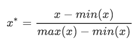
Data Normalization is generally called Normalization, also known as min max scaling. The formula is as follows:
Important parameters:
feature_range. This parameter controls the range to which we want to compress the data. It defaults to [0,1] and can also be changed to other ranges, such as [10,15].
Example:
 1 from sklearn.preprocessing import MinMaxScaler
 2 data = [[-1, 2], [-0.5, 6], [0, 10], [1, 18]]
 3 #Convert the data into a two-dimensional DataFrame for easier viewing
 4 #What would it look like to change to a watch?
 5 import pandas as pd
 6 pd.DataFrame(data)
 7 #Realize normalization
 8 scaler = MinMaxScaler() #instantiation
 9 scaler = scaler.fit(data) #fit, where the essence is to generate min(x) and max(x)
10 result = scaler.transform(data) #Export results through interface
11 result
12 result_ = scaler.fit_transform(data) #Training and export results are achieved in one step
13 scaler.inverse_transform(result) #The normalized results were reversed
14 #use MinMaxScaler Parameters of feature_range Normalize the data to[0,1]outside#In the range of
15 data = [[-1, 2], [-0.5, 6], [0, 10], [1, 18]]
16 scaler = MinMaxScaler(feature_range=[5,10]) #Still instantiate
17 result = scaler.fit_transform(data) #fit_transform one step export results
18 result
19 #When the number of features in X is very large, fit will report an error and say that the amount of data is too large for me to calculate
20 #Partial is used_ Fit as training interface
21 #scaler = scaler.partial_fit(data)
2,preprocessing.StandardScaler(x)
Definition:
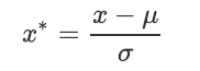
When data (x) is averaged( μ) After centralization, according to the standard deviation( σ) Scaling, the data will obey the normal distribution with mean value of 0 and variance of 1 (i.e. standard normal score)
And this process is called data Standardization (also known as Z-score normalization). The formula is as follows:
example:
 1 from sklearn.preprocessing import StandardScaler
 2 data = [[-1, 2], [-0.5, 6], [0, 10], [1, 18]]

 3 scaler = StandardScaler() #instantiation


 4 scaler.fit(data) #fit is essentially generating mean and variance
 5 scaler.mean_ #View the average attribute mean_
 6 scaler.var_ #View the variance attribute var_
 7 x_std = scaler.transform(data) #Export results through interface
 8 x_std.mean() #The result of the export is an array. Use mean() to view the mean value
 9 x_std.std() #Using std() to view variance


10 scaler.fit_transform(data) #Using fit_transform(data) achieves the result in one step
11 scaler.inverse_transform(x_std) #Use inverse_transform reverse standardization
3,processing.MinMaxScaler() and processing StandardScaler()
3.1 treatment of null NaN by two methods
For StandardScaler and MinMaxScaler, the null value NaN will be regarded as a missing value, which will be ignored during fit and transform
Maintain the status display of missing NaN. Moreover, although the de dimensioning process is not a specific algorithm, it is still allowed to import at least two dimensions in the fit interface
Group, one-dimensional array import will report an error. Generally speaking, the X we input will be our characteristic matrix. In real cases, the characteristic matrix is unlikely to be one-dimensional
So there won't be this problem.
3.2 which do you choose between StandardScaler() and MinMaxScaler()?
(1) it depends. In most machine learning algorithms, StandardScaler is selected for feature scaling because MinMaxScaler is very sensitive to outliers
Feeling. In PCA, clustering, logistic regression, support vector machine and neural network, StandardScaler is often the best choice.
(2) MinMaxScaler is widely used when it does not involve distance measurement, gradient, covariance calculation and data needs to be compressed to a specific interval, such as digital image
When quantifying pixel intensity in processing, MinMaxScaler will be used to compress the data in the [0,1] interval.
(3) it is recommended to try the StandardScaler first. If the effect is not good, change to MinMaxScaler.
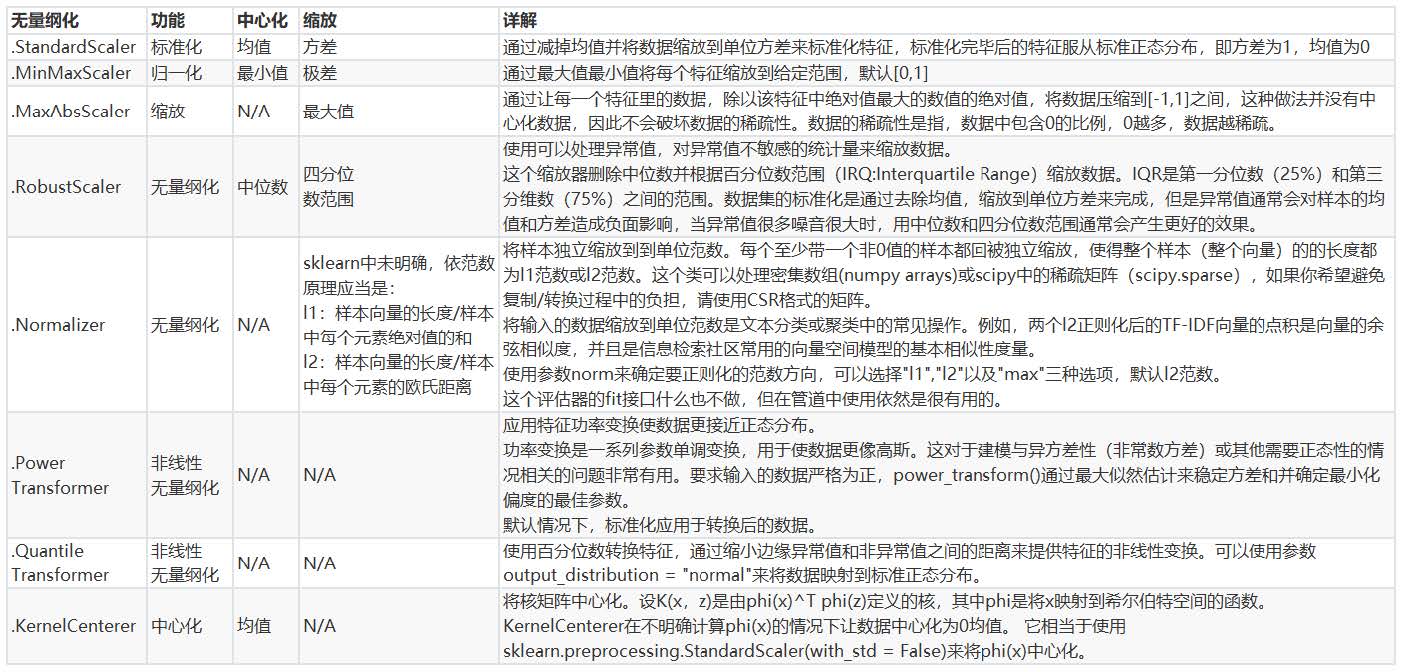
(4) in addition to the StandardScaler and MinMaxScaler, sklearn also provides various other scaling processing (centralization requires only one pandas)
Just play and subtract a certain number, so sklearn does not provide any centralization function). For example, when you want to compress data, it does not affect the sparsity of data
When the property does not affect the number of values of 0 in the matrix, we will use MaxAbsScaler; When there are many outliers and the noise is very large, we may choose
Dimensionless with quantile, RobustScaler is used. Please refer to the following list for more details.
II. Treatment of missing values
1. Why deal with missing values?
In machine learning, data can never be perfect. Without abandoning this feature, dealing with missing values is a very important item in the process of data preprocessing.
2. The function used in sklearn: impulse SimpleImputer()
Detailed explanation:
class sklearn.impute.SimpleImputer (missing_values=nan, strategy='mean', fill_value=None, verbose=0,copy=True)
Parameters:

3. Missing values can also be filled with Pandas and Numpy
1 import pandas as pd
2 data = pd.read_csv(r"C:\work\learnbetter\micro-class\week 3
3 Preprocessing\Narrativedata.csv",index_col=0)
4 data.head()
5 data.loc[:,"Age"] = data.loc[:,"Age"].fillna(data.loc[:,"Age"].median())
6 #. fillna directly fills in the DataFrame
7 data.dropna(axis=0,inplace=True)
8 #. dropna(axis=0) deletes all rows with missing values dropna(axis=1) deletes all columns with missing values
9 #Parameter inplace. If True, it means to modify the original dataset. If False, it means to generate a copy object without modifying the original data. The default is False
III. processing classification features: coding and dummy variables
1. Why deal with typed features?
In reality, many labels and features are not represented by numbers when the data is collected. For example, the value of educational background can be ["small"
Learn, "junior high school", "high school", "University", the payment method may include [Alipay, cash, WeChat] and so on. In this case, in order to make data fit
In response to algorithms and libraries, we must encode data, that is, convert literal data to numeric data.
sklearn specifies that numeric type must be imported.
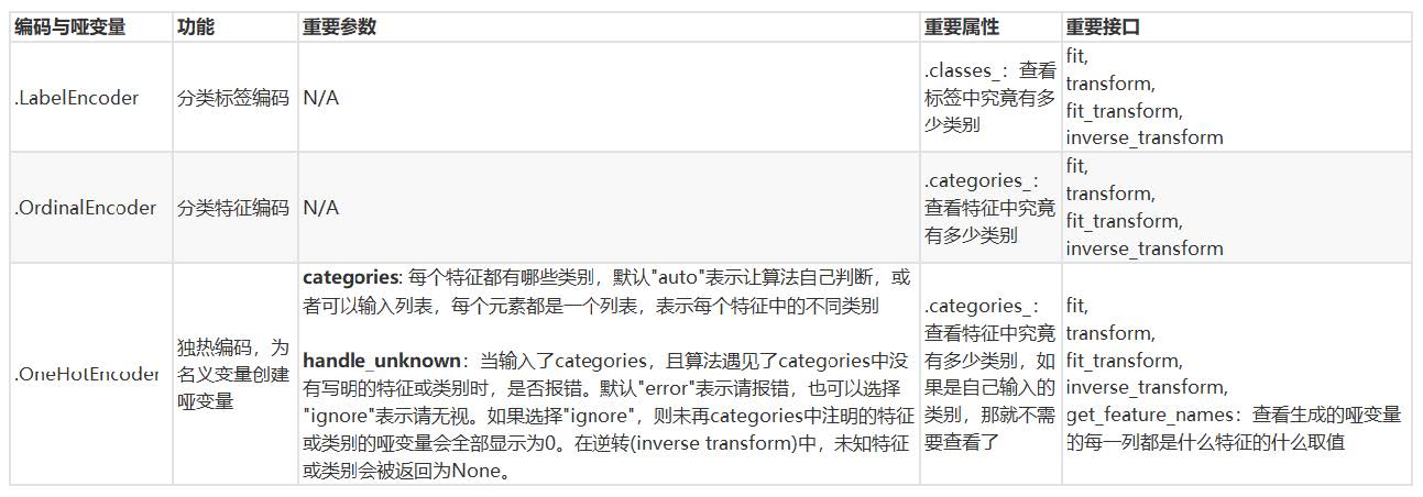
2,preprocessing.LabelEncoder: label specific, which can convert classification to classification value.
 1 from sklearn.preprocessing import LabelEncoder
 2 y = data.iloc[:,-1] #The label is to be entered, not the characteristic matrix, so one dimension is allowed
 3 le = LabelEncoder() #instantiation
 4 le = le.fit(y) #Import data
 5 label = le.transform(y) #The transform interface fetches the result
 6 le.classes_ #Properties classes_ See how many categories are in the label
 7 label #View the obtained results label


 8 le.fit_transform(y) #You can also directly fit_transform in one step
 9 le.inverse_transform(label) #Use inverse_transform can be reversed


10 data.iloc[:,-1] = label #Let the tag be equal to the result we run
11 data.head()

12 #If there is no need for teaching demonstration, I will write this:
13 from sklearn.preprocessing import LabelEncoder
14 data.iloc[:,-1] = LabelEncoder().fit_transform(data.iloc[:,-1])
3,preprocessing.OrdinalEncoder: feature specific, which can convert classification features into classification values.
1 from sklearn.preprocessing import OrdinalEncoder
2 #Interface categories_ Corresponding to LabelEncoder's interface classes_, As like as two peas
3 data_ = data.copy()
4 data_.head()
5 OrdinalEncoder().fit(data_.iloc[:,1:-1]).categories_
6 data_.iloc[:,1:-1] = OrdinalEncoder().fit_transform(data_.iloc[:,1:-1])
7 data_.head()
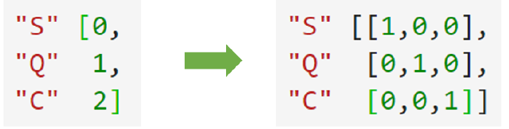
4,preprocessing.OneHotEncoder: single hot coding, creating dummy variables
4.1. Reasons for creating dummy variables:
When encoding features, these three classification data will be converted into [0,1,2]. In the view of the algorithm, these three numbers are continuous and can be used
Calculated, these three numbers are unequal to each other, have sizes, and have a connection that can be added and multiplied. So the algorithm will classify the hatch and education
Signs are misunderstood as classification characteristics such as weight. This means that when we convert classification into numbers, we ignore the mathematical properties inherent in numbers
To convey some inaccurate information to the algorithm, which will affect our modeling.
The category OrdinalEncoder can be used to handle ordered variables, but for nominal variables, we can only use dummy variables to handle them as much as possible
Convey the most accurate information to the algorithm: (see the figure below)
4.2 examples
 1 data.head()
 2 from sklearn.preprocessing import OneHotEncoder
 3 X = data.iloc[:,1:-1]
 4 enc = OneHotEncoder(categories='auto').fit(X)
 5 result = enc.transform(X).toarray()
 6 result
 7 #It can still be done directly in one step, but in order to show you the model properties, it is written in three steps
 8 OneHotEncoder(categories='auto').fit_transform(X).toarray()
 9 #Can still be restored
10 pd.DataFrame(enc.inverse_transform(result))
11 enc.get_feature_names()
12 result
13 result.shape
14 #axis=1 means cross row consolidation, that is, connecting the left and right of the gauge. If axis=0, connecting the top and bottom of the gauge
15 newdata = pd.concat([data,pd.DataFrame(result)],axis=1)
16 newdata.head()
17 newdata.drop(["Sex","Embarked"],axis=1,inplace=True)
18 newdata.columns =
19 ["Age","Survived","Female","Male","Embarked_C","Embarked_Q","Embarked_S"]
20 newdata.head()
4.3 labels can also be used as dummy variables
Use class sklearn preprocessing. Labelbinarizer can be used as a dummy variable for many algorithms
Deal with multi label problems (such as decision trees), but this is not common in reality.
4.4 summary
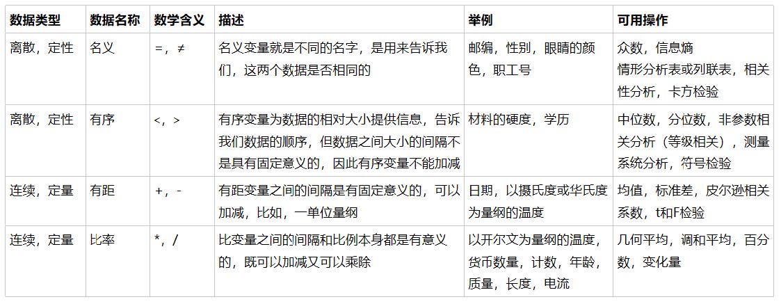
Attachment: data types and commonly used statistics
IV. processing continuous features: binarization and segmentation
1,sklearn.preprocessing.Binarizer ()
Explanation:
Binarize the data according to the threshold (set the eigenvalue to 0 or 1) for processing continuous variables. Values greater than the threshold map to 1 and less than or equal to the threshold
The value of the value is mapped to 0. When the default threshold is 0, all positive values in the feature are mapped to 1. Binarization is a common operation for text count data, which is difficult for analysts
It can be decided to consider only the existence of a phenomenon. It can also be used as a preprocessing step of an estimator considering Boolean random variables (e.g., using Bayes)
Bernoulli distribution modeling in settings).
example:
1 #Binarization of age
2 data_2 = data.copy()
3 from sklearn.preprocessing import Binarizer
4 X = data_2.iloc[:,0].values.reshape(-1,1) #Class is feature specific, so one-dimensional arrays cannot be used
5 transformer = Binarizer(threshold=30).fit_transform(X)
6 transformer
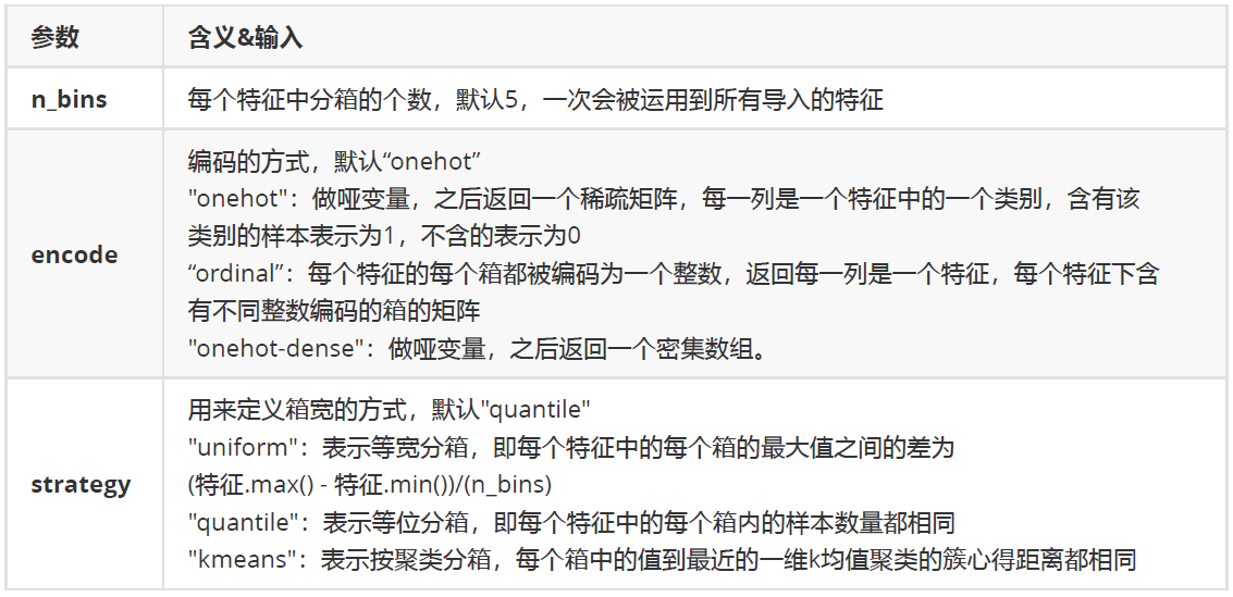
2,preprocessing.KBinsDiscretizer ()
Explanation:
This is a class that divides continuous variables into classified variables. Continuous variables can be sorted, boxed and coded in order. There are three important parameters:
example:
1 from sklearn.preprocessing import KBinsDiscretizer
2 X = data.iloc[:,0].values.reshape(-1,1)
3 est = KBinsDiscretizer(n_bins=3, encode='ordinal', strategy='uniform')
4 est.fit_transform(X)
5 #View the boxes divided after conversion: it becomes three boxes in a column
6 set(est.fit_transform(X).ravel())
7 est = KBinsDiscretizer(n_bins=3, encode='onehot', strategy='uniform')
8 #View the sub box after conversion: it has become a dummy variable
9 est.fit_transform(X).toarray()
End of this section!