1. Learn to use ndarray
1.1 What is ndarray?
ndarray is a multidimensional array object in NumPy that can be one-dimensional, two-dimensional, or even more.Of course, creating more dimensional arrays is not his advantage. Its advantage is that it has a rich method of operation, and it is also the base of another advanced Python library, pandas, but it can only store elements of the same type.
1.2 Create an ndarray
The first is to create ndarray directly from a list, as follows:
#The first is created directly from a list
a_list=[0,1,2,3,4]
a_ndarray=np.array(a_list)#Created a one-dimensional array
print(type(a_ndarray))
If you create a one-dimensional array above, you can also create a two-dimensional, three-dimensional array
Take a look at the following code:
c_list=[[0,0],[1,1,1],[2,2]]#This is an irregular two-dimensional list
c_ndarray=np.array(c_list)
print(c_ndarray)#Output Array
The output is: [list([0, 0]) list([1, 1, 1]) list([2, 2])]
Second, create an array of specified initial values for the specified shape
When we set an initial value of 0 or 1, we can use the functions zeros or ones to accept a tuple to represent the shape of the array.
The code is as follows:
#Creates the specified shape and initial value ndarray
d_ndarray=np.zeros(3)#Specify an initial value of 0 and a 1-D length of 3 for the initial shape
print(d_ndarray)
The output is: [0.0.0.] Here our element type is float
e_ndarray=np.ones((3,2))#Create an array of 3 rows and 2 columns
print(e_ndarray)
Create an N*N unit matrix using the eye function (diagonal 1, remaining 0)
f_ndarray=np.eye(3,3)#Create 3*3 Unit Matrix
print(f_ndarray)
1.3 Judging ndarray's shape and element type
Judging a ndarray shape uses the shape attribute of ndarray
e_ndarray=np.ones((3,2))
print(e_ndarray)
print(e_ndarray.shape)#Output Shape
The output is: (3, 2)
Determine the element type of an ndarray
e_ndarray=np.ones((3,2))
print(e_ndarray)
print(e_ndarray.dtype)#Type of output element
The output is: float64
Operation of 1.4 ndarray
Multiplication:
a_ndarray=np.array([[1,2,3],[4,5,6]])
b_ndarray=np.array([[7,8,9],[10,11,12]])
c_ndarray=a_ndarray*b_ndarray#Multiplication
print(c_ndarray)
Output: [[7 16 27]
[40 55 72]]
You can see that array multiplication is the multiplication of every element that traverses the array.
Subtraction:
a_ndarray=np.array([[1,2,3],[4,5,6]])
b_ndarray=np.array([[7,8,9],[10,11,12]])
c_ndarray=a_ndarray-b_ndarray#subtract
print(c_ndarray)
Output: [[-6-6-6]
[-6 -6 -6]]
Subtraction of corresponding elements
Reciprocal:
d_ndarray=1/a_ndarray #Reciprocal
print(d_ndarray)
Output: [[1.]0.5 * 0.333333]
[0.25 0.2 0.16666667]]
Power:.
e_ndarray=a_ndarray**2#Power
print(e_ndarray)
Output: [[1 4 9]
[16 25 36]]
Slices and copies of 1.5 ndarray
The difference between a ndarray slice and a list slice:
For list:
a_list=[1,2,3,4,5]
print(a_list) #First Output
b_list=a_list # Direct assignment
b_list[0]=0
print(a_list)  #Second Output
Output: [1, 2, 3, 4, 5]
[0, 2, 3, 4, 5]
It is found that by assigning a list directly, changing one of the other will also change.
a_list=[1,2,3,4,5]
print(a_list)#First Output
c_list=a_list[0:len(a_list)] # Using slices
c_list[0]=0
print(a_list)#Second Output
Output: [1, 2, 3, 4, 5]
[1, 2, 3, 4, 5]
We find that the list slice does not change the original element, that is, it completes a copy and passes the copied list to the new list
For ndarray slices:
a_list=[1,2,3,4,5]
a_ndarray=np.array(a_list)
b_ndarray=a_ndarray[0:len(a_list)]
print(a_ndarray)#First Output
b_ndarray[0]=9
print(a_ndarray)#Second Output
Output: [1 2 3 4 5]
[9 2 3 4 5]
We find that tile assignment in ndarray also simply creates a new reference to the original object.
Then the copy function is needed to copy in ndarray, as follows:
a_list=[1,2,3,4,5]
a_ndarray=np.array(a_list)
b_ndarray=a_ndarray.copy()
print(a_ndarray)#First Output
b_ndarray[:]=9
print(a_ndarray)#Second Output
Output: [1 2 3 4 5]
[1 2 3 4 5]
1.6 Array transpose:
# Transpose of arrays
import numpy as np
a_ndarray=np.array([[0,0,0],[1,1,1],[2,2,2]])
print(a_ndarray)
b_ndarray=a_ndarray.T#Transpose
print(b_ndarray)
Output: [[0 0 0]
[1 1 1]
[2 2 2]]
[[0 1 2]
[0 1 2]
[0 1 2]]
1.7 Operational functions accurate to element level
Common unary functions (functions that accept an array) are:
abs* Take absolute value
sqrt * prescription
Square * square
exp. Calculate the index of each element
Log log10 log2 The logarithmic base numbers are e, 10, 2, respectively
Return the minimum value greater than or equal to x
Return the maximum value less than or equal to x
rint Round each element to the nearest integer
isnan* Returns a bool array indicating which are arrays
sum
Mean * arithmetic mean
std var* Standard deviation variance
min max Maximum
sort* sort
Common binary functions (functions that accept two arrays) are:
add * add the corresponding elements of the two arrays
subtract The first array minus the second
multiply Array Elements
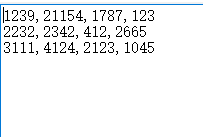
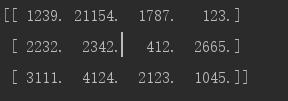
1.8 Transfer directly the contents of the txt file into the ndarray array
The data in the file can be imported into ndarray using the function loadtxt:

import numpy as np
a_ndaarray=np.loadtxt(r"E:\PythonWork\py Study\test",delimiter=',',encoding='GBK')
print(a_ndaarray)
The output is:

Similarly, the savetxt function stores an array in a txt file
Array (matrix) operations in 1.9 linear algebra
Returns a one-dimensional array representing the diag onal of a matrix
T) Matrix Transposition
dot* Matrix Multiplication
trace. Calculates the sum of the diagonal elements
det. Calculates the determinant of a matrix
eig) Compute the eigenvectors of a matrix
Origin: https://www.cnblogs.com/SAM-CJM/p/10152932.html