In our study of data structure, sorting is undoubtedly a very important algorithm. It should be described as an algorithm rather than a data structure. There will be many sorting algorithms in sorting. These sorting algorithms have their own advantages and disadvantages. They are designed with the wisdom of predecessors. There are many excellent ideas worth learning. Let's stand on the shoulders of giants, Let's learn about the 8 sorting algorithms

This paper draws lessons from some excellent pictures in @ 2021dragon's eight sorting algorithms (implemented in C language)

Basic concepts

Finally, add a non commutative sort to the count sort, and sort in a total of 8

Here, we analyze these eight sorting algorithms respectively

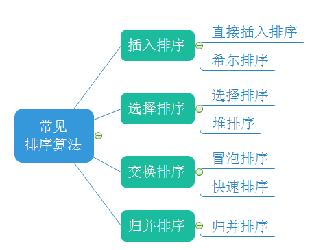
Direct insert sort

When inserting the I (I > = 1) th element, the preceding array[0],array[1],..., array[i-1] have been arranged in order. At this time, compare the sorting code of array[i] with the sorting code of array[i-1],array[i-2],... To find the insertion position, that is, insert array[i], and move the element order at the original position backward

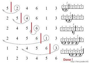
According to the above analysis, we can see that the essence of direct insertion sorting is to start from the second number and compare it with the first number. If it is small, the first number will move backward, the second number will be inserted to the front and iterate backward In the example above, in the process of array backward iteration, 2 is smaller than 5, 5 moves backward, 2 is inserted in front of 5, 4 is smaller than 5, 5 moves backward, 4 is inserted in front of 5, 6 is larger than 5, does not move, backward iteration, 1 is smaller than 6, smaller than 5, smaller than 4, smaller than 2, moves backward in turn, 1 is inserted in front of 2, 3 is smaller than 6, smaller than 5, smaller than 4, and inserted in front of 4 to complete sorting

Let's implement it in code

void InsertSort(int* a, int n)
{
	for (int i = 0; i < n - 1; i++){
		int end = i;//Defines the last subscript of an ordered sequence
		int tmp = a[end + 1];//Store the last value of end in tmp (the value to be inserted)
		while (end >= 0)//When end is still in the array
		{
			if (tmp < a[end])//If tmp value is smaller than end (forward interpolation is required)
			{
				a[end + 1] = a[end];//Move the value of the end subscript back to overwrite the original tmp position
				--end;//Continue checking forward
			}
			else{
				break;//Find the location to insert
			}
		}//Come here: 1 End has reached the - 1 position, tmp is smaller than all the previous numbers, and tmp is inserted into the subscript position 0
                    2.--end On the way, end Reduced to more than tmp Small value, find the place to insert
		a[end + 1] = tmp;//Insert the data stored in tmp into the last bit of end
	}
}

In general, it is to define an end subscript and a tmp variable to store the value to be inserted. The subscript is responsible for checking whether the position is correct. When the position is found, let the tmp value be placed in the correct position. The specific operation is that the outer end moves backward in turn, traverses from front to back, and the inner end traverses from back to front. Compared with tmp, tmp is small, and a[end]=a[end] value covers tmp position, End -- continue to look forward, tmp is small, continue to cover backward, and complete the move back operation. Finally, when the tmp is large, stop the cycle, insert tmp into the empty space, and then end and move tmp backward to insert the next number to complete the insertion sorting

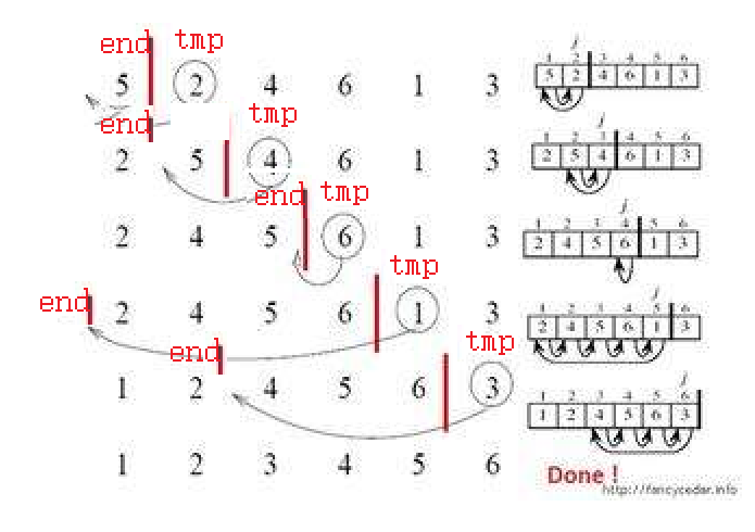
This is the relative position diagram of end and tmp when the last break finds the position. When the end moves forward but does not reach this relative position, the completed operation is to move the whole number between end and tmp backward by one bit. Finally, when end reaches the penultimate position of the array, that is, n-1, it is finished. This is our insertion sort

Shell Sort

When we complete the analysis of insertion sort, we will find that the time complexity of insertion sort will be reduced to O(N) when it is close to the order, and the time complexity will be O(N^2) when it is close to the reverse order. Therefore, in the research of insertion sort, Hill simulates to pre sort it first to make it close to the order as much as possible, and the sorting efficiency will be greatly improved. Therefore, Hill invented Hill sort. Hill sort is actually an optimization of insertion sort. It is a very excellent sort algorithm

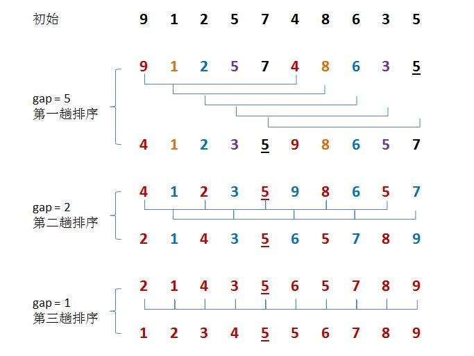
Hill's sorting idea is to perform insertion sorting by grouping first, because in ascending order, large numbers move to the back position, which requires many operations of covering and moving later. Moving one by one is too slow, so it introduces gap variables to allow big data to directly insert and sort later across gap units, which greatly reduces the consumption caused by moving one by one, For the above figure, let 9 and 4 be a group, 1 and 8 be a group, etc. insert and sort them respectively. After a round, the array is closer to order, and then group again to reduce the gap value. Let 4, 2, 5, 8, 7 and 5 be a group, and 1, 3, 9, 6 and 7 be a group. Insert and sort them again respectively. After the arrangement, it is closer to order, and finally reduce the gap again to make gap 1, At this time, the array is very close to order. Insert and sort the array to complete the sorting

We can find

When the gap is larger, the large and small numbers can move to the corresponding direction faster. The larger the gap, the less close to order

When the gap is smaller, the larger and smaller numbers can move to the corresponding direction more slowly. The larger the gap, the closer to order

When gap is 1, it is our insertion sort, so we need to make gap as large as possible, finally make gap small, and finally reach 1

The following is our code implementation

void ShellSort(int *a, int n)
{
	int gap = n;//Set initial value for gap
	while (gap > 1)//Pre sort when gap is greater than 1
	{
		gap = (gap / 3 + 1);//Here we choose / 3 for reduction
	}
	for (int i = 0; i < n - gap; i++)//Start sorting in sequence, i change a group of numbers apart from gap for every + 1, until it reaches the position of n-gap
	{
		int end = i;
		int tmp = a[end + gap];
		while (end >= 0)
		{
			if (tmp < a[end])
			{
				a[end + gap] = a[end];
				a -= gap;
			}
			else
			{
				break;
			}
		}
		a[end + gap] = tmp;
	}
}

For this code, changing gap to 1 in the lower loop is our insertion sort. The operation we do in the outer layer is that for each additional i, the array will be cut to the next group for sorting

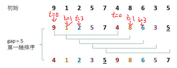
As shown in the figure above, when i=1, insert sort 9,4, and when i=2, insert sort 1,8 until i reaches position n-gap=5 and stops when the subscript is 4. A round of insert sort is completed. When gap is reset, insert and sort more data again, and finally gap is 1 to complete Hill sort

Select sort

In fact, the idea of selecting sorting is very simple. Go through the whole array, select the smallest one and put it in subscript 0, then traverse the remaining n-1 elements, select the smallest one and put it in subscript 1, and so on until the outer layer traverses the whole array

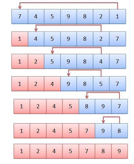
For the above array, traverse the whole array from 7 to 1, find the smallest 1, exchange 1 with 7 of subscript 0, traverse 4 to 7, find the smallest 2, exchange with 4 of subscript 1, and finally traverse 9 to 8, find the exchange of small 8 with 9 of subscript 6, and complete the sorting

Let's implement it in code

//Select sort (one at a time)
void SelectSort(int* a, int n)
{
	int i = 0;
	for (i = 0; i < n; i++)//i represents the subscript of the first element participating in the selection sorting of the trip
	{
		int start = i;
		int min = start;//Record the subscript of the smallest element
		while (start < n)
		{
			if (a[start] < a[min])
				min = start;//Subscript update of minimum value
			start++;
		}
		Swap(&a[i], &a[min]);//The minimum value exchanges positions with the first element participating in the selection sort of the trip
	}
}

void SelectSort(int *a, int n)(Two numbers at a time)
{
	int left = 0; int right = n - 1;//Set the maximum and minimum flag positions at the left and right ends
	while (left < right)
	{
		int minIndex = left, maxIndex = right;
		for (int i = left; i <= right; i++)//Scan the middle non maximum and minimum interval
		{
			if (a[i] < a[minIndex])//Find the minimum value and store its subscript in minIndex
				minIndex = i;
			if (a[i] > a[maxIndex])//Find the maximum value and store its subscript in maxIndex
				maxIndex = i;
		}
		Swap(&a[left], &a[minIndex]);//Swap the minimum value with left
		if (left == maxIndex)//It is excluded that when the maximum value is in the left position, because max has changed after exchanging with min in the previous step, and then the following exchange is affected
		{
			maxIndex = minIndex;
		}
		Swap(&a[right], &a[maxIndex]);//
		++left;
		--right;
	}
}

Note that the code implementation here is to sort the maximum value and the minimum value at the same time, rather than just the minimum value, which can greatly improve the efficiency. However, there is an additional point to pay attention to at the exchange, which needs to be handled separately for the case of left==max. we will show the results not handled below

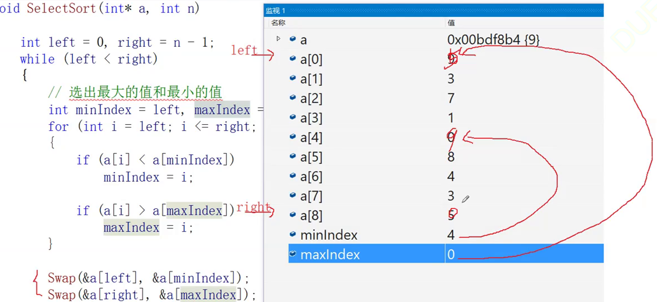
We can see that when left==max, left is subscript 0, min is subscript 4, right is subscript 8, and Max is subscript 0. Then left first exchanges with min, subscript 0 becomes the number of subscript 4, and then right exchanges with Max, and subscript 8 becomes the number of subscript 0, However, at this time, the number of subscript 0 has been replaced by the number of subscript 4 in the previous step, so it is no longer the maximum value, and Max has been changed in the previous step. Therefore, when we encounter this situation, we can assign min to Max and reassign the original maximum to solve the problem

Heap sort

Before we know about heap sorting, we must first understand an important algorithm in the heap building process, the downward adjustment algorithm. As the name suggests, the downward adjustment algorithm, take the heap building process as an example

1. Premise: the subtrees on both sides are a lot, but the root node does not conform to the lot

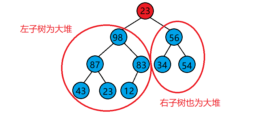
 2. Method: scan the heap. If the parent node is smaller than the left and right leaf nodes, exchange the large one of the left and right child trees with the parent node and recurse downward until the original parent node reaches the leaf node or when both the left and right child trees are smaller than him in the recursion process, stop the adjustment and complete the adjustment

 3. Effect: the operation completed by this algorithm is to turn the left and right subtrees into a large heap, adjust the whole heap into a large heap, adjust the root node to its position, and maintain the integrity of the heap

Let's implement the code

void AdjustDown(int *a, int n, int parent)//Array pointer, number of array elements, parent node variable
{
	int child = parent * 2 + 1;//Define the relationship between the left child and the father (child + 1 for the right child)
	while (child < n){//When the child node is in the array (when the child does not exist, the father goes to the leaf node)
		if (child + 1 < n&&a[child + 1] < a[child]){//The right child exists and the right child is small (the left child is small by default)
			++child;//So let the little child become the right child
		}
		if (a[child] < a[parent]){//When the child is smaller than the father (note that the left and right children are not distinguished here, because the result obtained by dividing the left and right children in the calculation is the same)
			Swap(&a[parent],&a[child]);//Exchange children and fathers
			parent = child;//Children become new fathers
			child = parent * 2 + 1;//Restore the relationship between the child and the father,
		}
       else{
              break;//If it meets the requirements, you can exit directly without adjustment
        }
	}
}

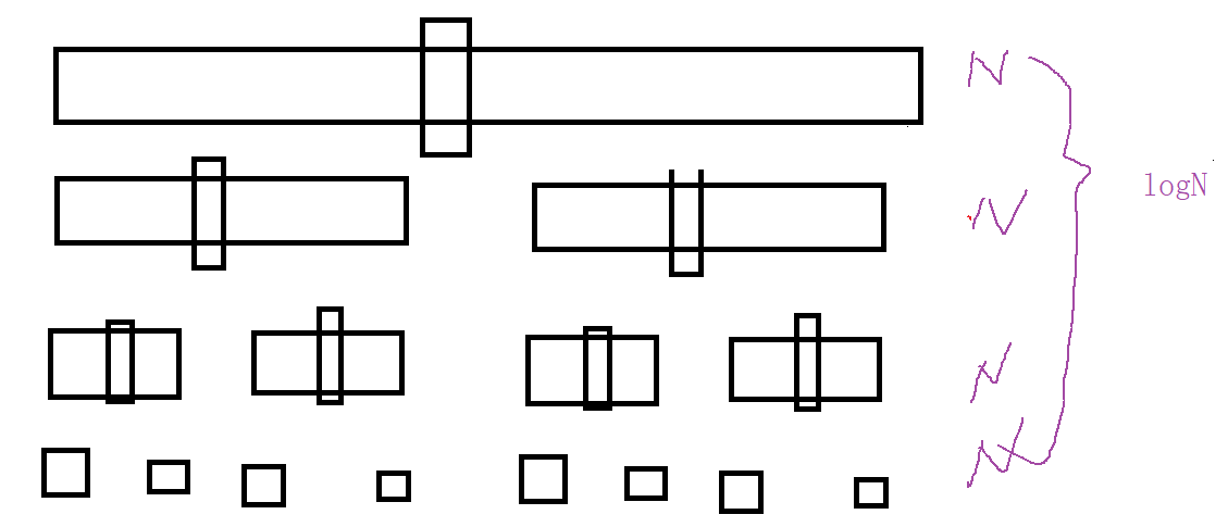
We can see that the heap down adjustment algorithm, after adjusting a heap, requires a maximum time complexity of tree height, so its time complexity is O(logN), which is an excellent algorithm

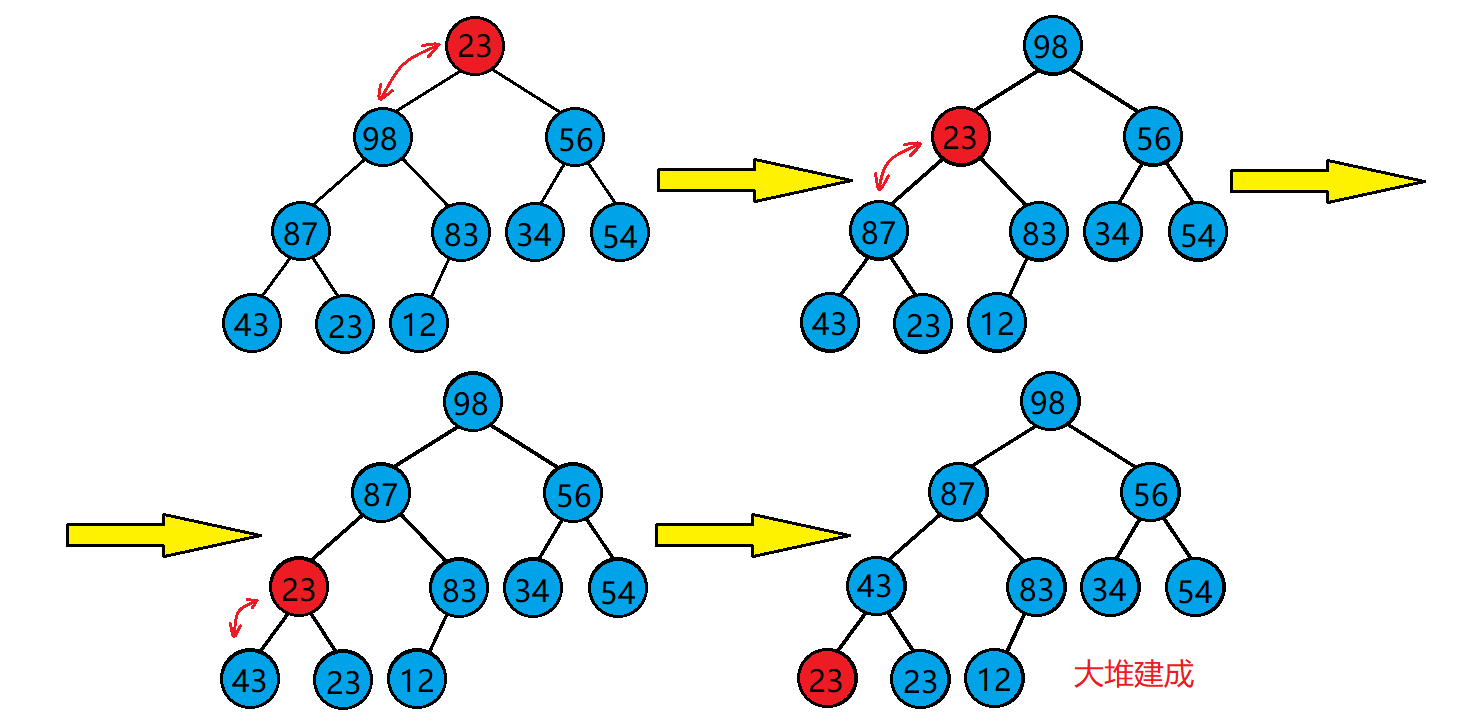
Then, after we understand the downward adjustment algorithm, we know that this algorithm can only adjust the heap of two subtrees into a complete heap, not for any complete binary tree, so how can we adjust any complete binary tree into a heap? At this time, we need to adjust it from bottom to top in turn

That is, as shown in this figure, adjust it from bottom to top, and finally it can be adjusted to a standard one

Let's implement this step in code

for (int i = (n - 1 - 1) / 2; i >= 0; i++)//Find the first non leaf node
	{
		AdjustDown(a, n, i);
	}

Here is the process of building a heap for any complete binary tree

Let's move on to our topic, heap sorting

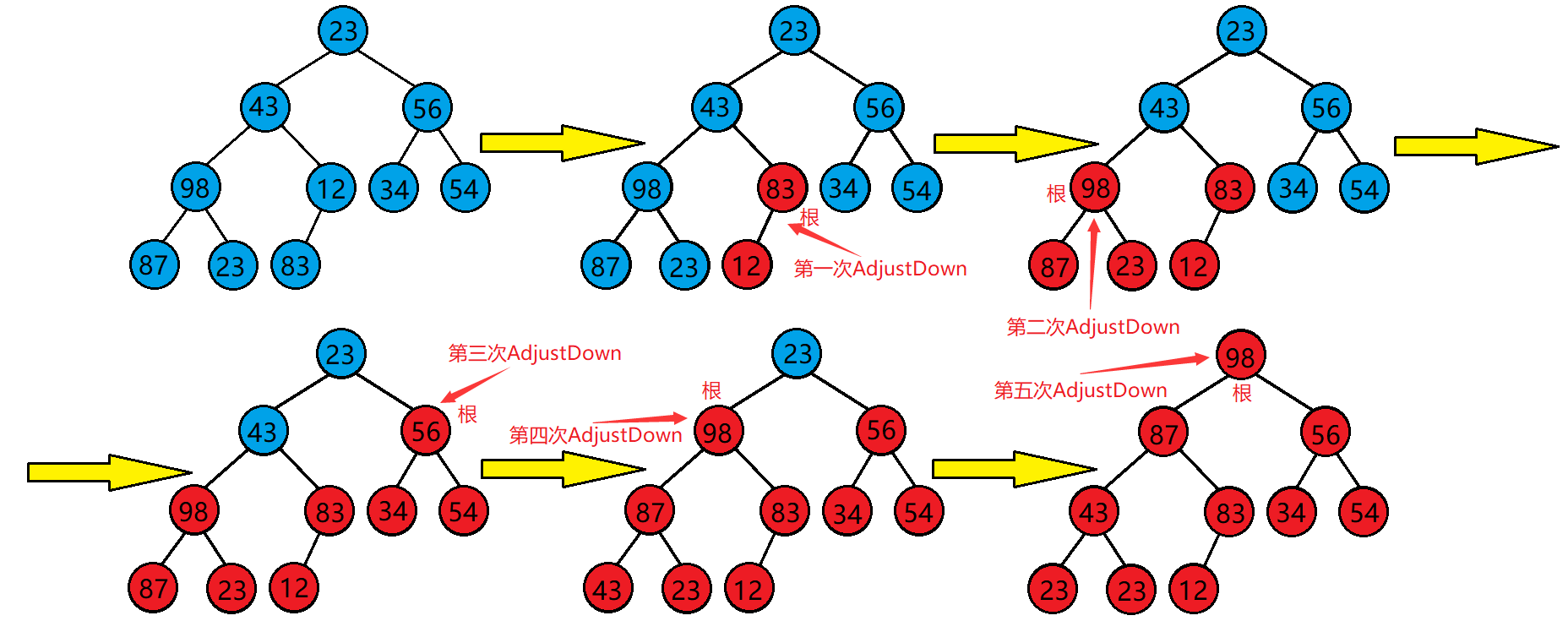
Heap sorting is to sort a group of data by using the data structure heap. When we need to sort a group of data in ascending order, we need to create a lot. At this time, the maximum number is at the top root node, and then exchange the root node with the last node. After the exchange, ignore the maximum number at the last node. For other numbers, It is also a complete binary tree with a large number of two children. At this time, build a heap for other numbers except the maximum number to get a new heap, and then exchange the root node with the maximum number to repeat the above process

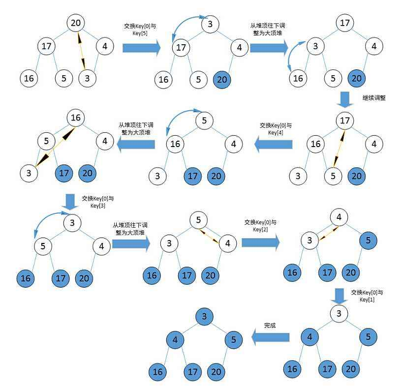
Just like this figure, continue to build a heap on the white part, find the maximum number, ignore, build a heap, ignore again, and finally complete the heap sorting

Let's show the overall code of heap sorting

void Swap(int *a, int *b)//Exchange function
{
	int temp = *a;
	*a = *b;
	*b = temp;
}
void AdjustDown(int *a, int n, int parent)//Array pointer, number of array elements, parent node variable
{
	int child = parent * 2 + 1;//Define the relationship between the left child and the father (child + 1 for the right child)
	while (child < n){//When the child node is in the array (when the child does not exist, the father goes to the leaf node)
		if (child + 1 < n&&a[child + 1] < a[child]){//The right child exists and the right child is small (the left child is small by default)
			++child;//So let the little child become the right child
		}
		if (a[child] < a[parent]){//When the child is smaller than the father (note that the left and right children are not distinguished here, because the result obtained by dividing the left and right children in the calculation is the same)
			Swap(&a[parent],&a[child]);//Exchange children and fathers
			parent = child;//Children become new fathers
			child = parent * 2 + 1;//Restore the relationship between the child and the father,
		}
       else{
              break;
        }
	}
}
void HeapSort(int* a, int n)//Array pointer, number of array elements
{
	//Build pile
	for (int i = (n - 1 - 1) / 2; i >= 0; --i)//Build the reactor from bottom to top
	{
		AdjustDown(a, n, i);
	}
	int end = n - 1;
	while (end > 0)//Keep putting numbers in the right place from back to front
	{
		Swap(&a[0], &a[end]);
		//Choose the next largest
		AdjustDown(a, end, 0);//Adjust downward from end, ignore the number arranged, and readjust other numbers
		end--;
	}
}

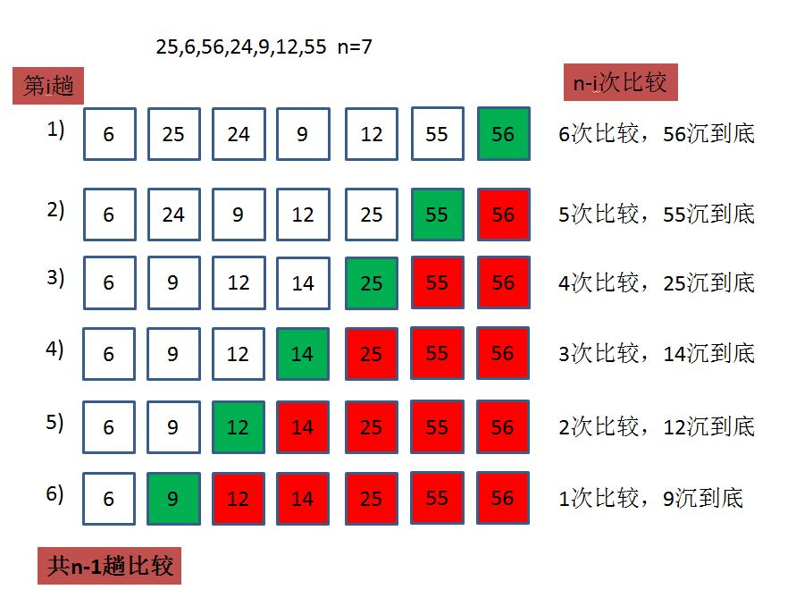
Bubble sorting

We used to be familiar with bubble sorting, that is, like bubbles in water, big bubbles always come out first, one by one

Let's implement the code below

void BubbleSort(int* a, int n)
{
	int end = 0;//First ordinal subscript
	for (end = n - 1; end >= 0; end--)
	{
		int exchange = 0;//Record whether the bubble sort has been exchanged
		for (int i = 0; i < end; i++)
		{
			if (a[i]>a[i + 1])
			{
				Swap(&a[i], &a[i + 1]);
				exchange = 1;
			}
		}
		if (exchange == 0)//The bubbling sort has not been exchanged, and there is an order
			break;
	}
}

Quick sort

For quick sorting, the essence is to select an intermediate value so that the number on the left of the intermediate value is less than him and the number on the right is greater than him, and then select the intermediate value again for the left and right intervals, divide them left and right, and finally finish sorting

Hoare method

The main step of Hoare method is to set the left and right pointers first, and then move the left and right pointers to the middle respectively. When the left pointer encounters a number larger than the middle value, it stops, and the right pointer encounters a stop smaller than the middle value, then exchange the numbers of the two stopped pointers, move closer to the middle again, and repeat the above process until the two pointers meet, Finally, exchange the middle value with the value at the position where the two pointers meet, and complete the operation that the number on the left is less than the middle value and the number on the right is greater than the middle value

When we finish sorting in a single run, we just need to repeat this operation on the left and right sides of the sorted key until the number of sorting is one or the end is reached

Implementation of recursive code for rapid sorting of Hoare method

void QuickSort1(int* a, int begin, int end)//Array pointer, start position, end position
{
	if (begin >= end)//Exits when the array has only one element or does not exist
		return;
	int left = begin;//Initialize left pointer
	int right = end;//Initialize right pointer
	int key = left;//Initialize key pointer
	while (left < right)//Start cycle
	{
		while (left < right&&a[right] >= a[key])//right go first and find something smaller than key
		{
			right--;//right shift left
		}
		while (left < right&&a[left] <= a[key])//left, go back and find something bigger than key
		{
			left++;//left shift right
		}
		if (left < right)//When the left position value is larger than the key, the right position value is smaller than the key
		{
			Swap(&a[left], &a[right]);//exchange
		}
	}
	int meet = left;//After completing the cycle, record the subscript at the time of encounter
	Swap(&a[key], &a[meet]);//exchange
	QuickSort1(a, begin, meet - 1);//Recursive fast row on the left
	QuickSort1(a, meet + 1, end);//Recursive fast row on the right
}

Excavation method

For the pit digging method, the main idea is to first store the value of the key, and then the left pointer and the right pointer, like the Hoare method, respectively look for the numbers in the corresponding range. However, the pit digging method is different. When the right pointer finds the decimal, it fills the decimal to the position where we start the key. The pit becomes the position of right at this time, and then let the left go to find the large number, Fill the large number into the pit at this time (right position), and then change the left position into a pit, so as to cycle until they meet. Finally, fill the key into the pit at the time of meeting

The effect of this method is that the values on the left side of the key are less than the key, and the values on the right side are greater than the key

The following is the code implementation of the excavation method

void QuickSort2(int* a,int begin, int end)
{
	if (begin >= end)
		return;
	int left = begin;
	int right = end;
	int key = a[left];//Store the leftmost value in key
	while (left < right)
	{
		while (left < right&&a[right] >= key)
		{
			right--;
		}
		a[right] = a[left];//Fill the small value into the pit
		while (left < right&&a[left] <= key)
		{
			left++;
		}
		a[right] = a[left];//Fill the large value into the pit
	}
	int meet = left;//Assign the meeting point as meet
	a[meet] = key;//Fill the key into the pit

	QuickSort2(a, begin, meet - 1);
	QuickSort2(a, meet + 1, end);
}

Front and back pointer method

Previously, we used the strategy of moving the left and right sides to the middle respectively, and the front and back pointer rule is to start from left to ensure that the middle part of prev to cur is greater than the key, and the left to prev is less than the key until cur comes out of the array

We can see that at the beginning, the interval between prev and cur is 1. Cur goes first. When the value pointed to by cur is smaller than the key, prev + + and cur exchange, and do not exchange when it is larger. Finally, until cur goes out of the array, all values less than the key are between left and prev, and values greater than the key are between cur and prev

Let's demonstrate the code

int QuickSort3(int* a, int left, int right)
{
	int midIndex = GetMidIndex(a, left, right);//Get the intermediate value from the three values
	Swap(&a[left], &a[midIndex]);//Assign an intermediate value to left
	int key = left;//Initialize key pointer
	int prev = left, cur = left + 1;//Initializing prev and cur pointers
	while (cur < right)//Start cycle
	{
		if (a[cur] < a[key])//When cur value is smaller than key
		{
			Swap(&a[cur], &a[prev++]);//cur and prev + + exchange
		}
		++cur;
	}
	Swap(&a[key], &a[prev]);//Finally, the intermediate value is exchanged with prev
}

When we write this method, we use an optimization method, three data fetching. Next, we will introduce two optimization methods of quick sorting

Fast scheduling optimization

For our quick sorting, the selection of key value greatly affects the sorting efficiency. When the key value is in the middle, the execution times of quick sorting tend to logN*N. however, when it is on both sides, the efficiency will be greatly reduced and close to N*N

When the key value approaches the middle median, the recursion depth is logN. The closer it is to dichotomy, the higher the efficiency

When approaching both sides, the depth approaches N, and the time complexity degenerates into bubbling

Triple median

As the name suggests, the middle of the three numbers is taken. We might as well imagine that when the value of the key in an array reaches the minimum or maximum value, it means that the remaining n-1 numbers are reordered, and the efficiency is the lowest. Therefore, in order to avoid the key getting to the end point value, we introduce the optimization method of three numbers

The idea of triple counting is to take the first, last and middle values in the array, select the middle value from the three values, and return its subscript

Let's demonstrate the code

int GetMidIndex(int* a, int left, int right)
{
	int mid = (left + right) >> 1;
	if (a[left] < a[mid])//When left is smaller than mid
	{
		if (a[mid] < a[right])
		{
			return mid;
		}
		else if (a[left] > a[right])
		{
			return left;
		}
		else
		{
			return right;
		}
	}
	else//When left is larger than mid
	{
		if (a[mid] > a[right])
		{
			return mid;
		}
		else if (a[left] < a[right])
		{
			return left;
		}
		else
		{
			return right;
		}
	}
}

In fact, for the three number middle algorithm, we take three numbers and find the middle size. It's relatively simple

Inter cell optimization

When we perform recursive fast scheduling, when the depth of recursion is very deep and the value of each recursive interval is very small, we still need to call recursion many times to complete the sorting, and recursion is a more expensive algorithm. Can we stop recursion when the number of elements in recursion decreases to a certain number, Instead, the remaining few numbers are sorted by other sorting algorithms without calling recursion, which can improve a certain efficiency, but the efficiency improvement is not as big as the middle of the three numbers

//Optimized quick sort
void QuickSort0(int* a, int begin, int end)
{
	if (begin >= end)//When only one data or sequence does not exist, no operation is required
		return;

	if (end - begin + 1 > 20)//Self adjustable
	{
		//You can call any of the three types of single pass sorting of quick sort
		//int keyi = PartSort1(a, begin, end);
		//int keyi = PartSort2(a, begin, end);
		int keyi = PartSort3(a, begin, end);
		QuickSort(a, begin, keyi - 1);//The left sequence of key is used for this operation
		QuickSort(a, keyi + 1, end);//The right sequence of key is used for this operation
	}
	else
	{
		//HeapSort(a, end - begin + 1);
		ShellSort(a, end - begin + 1);//Hill sort is used when the sequence length is less than or equal to 20
	}
}

We can control the remaining number of the last cancelled recursive interval, and we can also control other sorting algorithms used last to improve efficiency

At present, quick sorting with optimization algorithm is the fastest of all sorting algorithms

Non recursive implementation of fast scheduling

We know that when a recursive function is too deep, the stack space may be insufficient. At this time, we need non recursive writing to complete the implementation of fast scheduling. Non recursive writing is also called iterative writing. The efficiency of iteration is better than recursion in most cases. Although it is relatively complex, it is also something we must master

void QuickSortNonR(int* a, int begin, int end)
{
	Stack st;//Create stack
	StackInit(&st);//Initialization stack
	StackPush(&st, begin);//L to be sequenced
	StackPush(&st, end);//R to be sequenced
	while (!StackEmpty(&st))
	{
		int right = StackTop(&st);//Read R
		StackPop(&st);//Out of stack
		int left = StackTop(&st);//Read L
		StackPop(&st);//Out of stack
		//The single pass sorting of Hoare version is called here
		int keyi = PartSort1(a, left, right);
		if (left < keyi - 1)//The left sequence of the sequence also needs to be sorted
		{
			StackPush(&st, left);//L stack of left sequence
			StackPush(&st, keyi - 1);//R stack of left sequence
		}
		if (keyi + 1 < right)// The right sequence of the sequence also needs to be sorted
		{
			StackPush(&st, keyi + 1);//L stack of right sequence
			StackPush(&st, right);//R stack of right sequence
		}
	}
	StackDestroy(&st);//Destroy stack
}

In fact, for any recursive iteration, we need to borrow the stack, and then cycle to calculate the recursive start point and stop point, put the start point and stop point into the stack, and then the stop point and start point out of the stack, call fast row, and then calculate the start points and stop points on both sides, read, out of the stack, repeat the operation, that is, save the recursive boundary in the form of stack, and then read it out for use

1. The overall comprehensive performance and usage scenarios of quick sort are relatively good, so I dare to call it fast sort

2. Time complexity: O(N*logN)

 

Merge sort

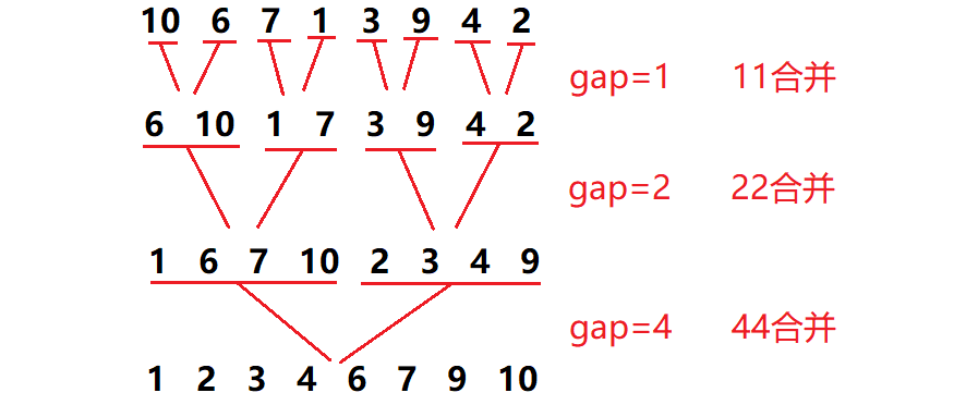
Merge and sort, using the idea of divide and rule, first separate large intervals, then sort each cell, and finally merge. The specific operation is shown in the figure below. First separate the array layer by layer, then merge two by two, merge four by four, and finally merge into a large interval, and complete the sorting on the way of merging

Let's implement it in recursive code

void _MergeSort(int* a, int left, int right, int* tmp)
{
	if (left >= right)//Returns when the interval has no elements
		return;

	int mid = (left + right) >> 1;//Find interval intermediate value
	// [left, mid][mid+1,right] the interval needs to be sorted
	_MergeSort(a, left, mid, tmp);
	_MergeSort(a, mid+1, right, tmp);

	// Two ordered subintervals are merged into tmp and copied back
	int begin1 = left, end1 = mid;//Left subinterval
	int begin2 = mid+1, end2 = right;//Right subinterval
	int i = left;//Total interval initial subscript
	while (begin1 <= end1 && begin2 <= end2)//Put the small interval into tmp
	{
		if (a[begin1] < a[begin2])
			tmp[i++] = a[begin1++];
		else
			tmp[i++] = a[begin2++];
	}

	while (begin1 <= end1)//Copy the remaining values of the two intervals into tmp
		tmp[i++] = a[begin1++];

	while (begin2 <= end2)
		tmp[i++] = a[begin2++];

	// After merging, copy back to the original array
	for (int j = left; j <= right; ++j)
		a[j] = tmp[j];
}

void MergeSort(int* a, int n)
{
	int* tmp = (int*)malloc(sizeof(int)*n);//Create temporary array
	if (tmp == NULL)
	{
		printf("malloc fail\n");
		exit(-1);
	}

	_MergeSort(a, 0, n - 1, tmp);

	free(tmp);//Release temporary array
}

The main idea is to copy the two intervals into tmp for sorting, and finally copy the data in tmp back to the original array

What about our non recursive approach

Non recursive merge sort

In the merge sort, the length of the merge interval is in a regular and continuous reduction process, and will eventually converge into a number of group leaders. Therefore, for our non recursive merge sort, we do not need to use the stack, but only need to control the length of the merge interval

When we use this method with fixed interval length, we inevitably need to consider the remaining three cases

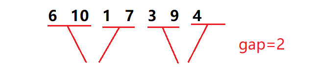
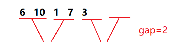
We need to deal with it separately

Here is our iterative approach

void _Merge(int* a, int* tmp, int begin1, int end1, int begin2, int end2)
{
	int j = begin1;
	int i = begin1;
	while (begin1 <= end1 && begin2 <= end2)
	{
		if (a[begin1] < a[begin2])
			tmp[i++] = a[begin1++];
		else
			tmp[i++] = a[begin2++];
	}

	while (begin1 <= end1)
		tmp[i++] = a[begin1++];

	while (begin2 <= end2)
		tmp[i++] = a[begin2++];

	// After merging, copy back to the original array
	for (; j <= end2; ++j)
		a[j] = tmp[j];
}


void MergeSortNonR(int* a, int n)
{
	int* tmp = (int*)malloc(sizeof(int)*n);//Open tmp array
	if (tmp == NULL)
	{
		printf("malloc fail\n");
		exit(-1);
	}

	int gap = 1;//Set initial value of interval length
	while (gap < n)//Start cycle
	{
		for (int i = 0; i < n; i += 2 * gap)//Jump to the next interval each time
		{
			// [i,i+gap-1][i+gap, i+2*gap-1] merging (when I increases, the number of intervals also increases. These two formulas can always represent the former interval and the latter interval)
			int begin1 = i, end1 = i + gap - 1, begin2 = i + gap, end2 = i + 2 * gap - 1;

			// If the second cell does not exist, there is no need to merge. End this cycle
			if (begin2 >= n)
				break;

			// If there are gaps in the second cell, but there are not enough gaps in the second cell, the end position is out of bounds and needs to be corrected
			if (end2 >= n)
				end2 = n - 1;

			_Merge(a, tmp, begin1, end1, begin2, end2);//Merge and sort intervals
		}

		gap *= 2;//Double each interval
	}

	free(tmp);//Free empty array
}

Count sort

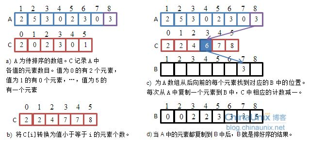
Our previous sorting is comparative sorting, which obtains the order by comparing the size of two numbers, while count sorting is a non comparative sorting, which uses the original subscript of the array to record data

For the data in the above figure, count and sort the original array by using another new array to scan and record the number of the same data. If 0 appears twice, the number of subscript 0 in the new array is 2. If 1 does not appear, the number of subscript 1 is 0... If the maximum value 5 appears once, the last subscript 5 in the new array is 1, Then copy the number of elements * corresponding to each element in the new array back to the original array to complete the sorting

This way that 1 corresponds to subscript 1 and 2 corresponds to subscript 2 is called absolute mapping

Besides this, what if you want to sort the following arrays

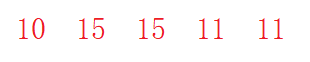
They are all numbers greater than 10 and less than 15. At this time, we need to open up an additional grid. Because the minimum value is 10 and the maximum value is 15, we open an array of size 7. The last subscript 6 is used to store 10, which means that these numbers need to be added with 10 to be their original size. This mapping method is called relative mapping, The difference is that a maximum common unit 10 is also added

Let's implement this sort method in code

// Time complexity: O(N+range)
// It is only suitable for a group of data, and the range of data is relatively centralized If the scope is concentrated, the efficiency is very high, but the limitations are also here
// And only suitable for integers, if it is a floating point number, string, etc
// Spatial assistance: O(range)
void CountSort(int* a, int n)
{
	int max = a[0], min = a[0];//Initialization max, min
	for (int i = 0; i < n; ++i)//Scan the array to get max, min
	{
		if (a[i] > max)
			max = a[i];

		if (a[i] < min)
			min = a[i];
	}

	int range = max - min + 1;//Get the size of the new array that needs to be opened up
	int* count = malloc(sizeof(int)*range);//Open up a new array
	memset(count, 0, sizeof(int)*range);//initialization
	for (int i = 0; i < n; ++i)//Scan the original array and copy the number of elements to the new array
	{
		count[a[i] - min]++;
	}

	int i = 0;
	for (int j = 0; j < range; ++j)//Copy the values of the new array back to the original array
	{
		while (count[j]--)
		{
			a[i++] = j + min;
		}
	}

	free(count);//Release new array
}

Sort summary

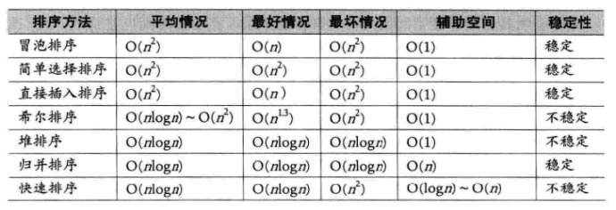
When we need to judge the stability of the sorting algorithm, we only need to recall whether there is jumping number exchange in the sorting process of each sorting algorithm. When two identical numbers can ensure that the relative position relationship remains unchanged before and after sorting, they are stable