//I can also liver again// I can't finish crying
Graph structure is a more complex nonlinear structure than tree structure, and any two terms may be related.
Logical structure of graph
definition
Vertices: data elements in a graph
Graph: it consists of a finite nonempty set of vertices and a set of edges between vertices.

Undirected edge: there is no direction between two vertices. (𝑣𝑖,𝑣𝑗)
Directed edge: there is a direction between two vertices. Ordered even pair representation< 𝑣, 𝑣, 𝑗 >, 𝑣, arc tail, arc head
catalogue
Adjacency matrix vs adjacency table
Undirected graph: the edge between any two points is an undirected edge.
Directed graph: the edge between any two points is a directed edge.
Weight: a meaningful numerical quantity assigned to an edge.
Weighted graph (net graph): a graph with weights on the edges.
Basic terms
1. Adjacency: if any two vertices have edges, the two vertices are adjacent to each other.

Penetration: the number of arcs whose vertices are arc heads. (enter this vertex)
Out degree: the number of arcs whose vertices are arc tails. (out of this vertex)
Out = in = number of edges
3. Undirected complete graph: any two points have edges.
Directed complete graph: any two points have two arcs with opposite directions.
4. Sparse graph: few edges.
Dense graph: many edges.
5. Path: a vertex sequence from one vertex to another.
Path length: the number of edges on the path.
Loop: first vertex = path of last vertex.
6. Simple path: a path where vertices do not appear repeatedly.
Simple loop: a loop in which vertices do not reappear except the first and last vertices.
7. Subgraph: a graph whose vertices belong to the original vertex set and whose edges belong to the original edge set. A graph can have multiple subgraphs.
8. Connectivity: if there is a path between two points in an undirected graph, the two points are connected.
Connected graph: there is a path between any two vertices.
Connected component: the polar connected subgraph of a non connected graph.
9. Strongly connected graph: in a directed graph, there is a path between any two vertices.
Strongly connected components: maximal strongly connected subgraphs of non strongly connected graphs.
Abstract data type definition of diagram:
The finite set of vertices and the set of edges between vertices, the establishment of graphs, the destruction of graphs, depth first traversal, breadth first traversal.
Traversal of Graphs
Starting from a vertex in the graph, all vertices in the graph are accessed once and only once.
There is no definite starting vertex in the graph. You can start from any vertex in the graph and number the vertices from 0.
In the process of traversal, distinguish whether the vertex has been accessed: set an access flag array visited[n], and the initial values are 0, indicating that it has not been accessed. If a vertex I is accessed, then visited[i]=1.
Depth first traversal
Recursive way
It is similar to the preorder traversal of a tree.
1. Access vertex v
2. Select a vertex w from the unreachable adjacency points in v, and then start from w for depth first traversal
3. Repeat 1 2
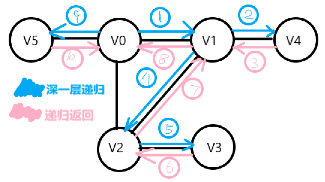
breadth-first search
Sequence traversal similar to a tree.
1. Access vertex v
2. Access each unreachable adjacency point w,x of v in turn
3. From w,x Start by visiting the adjacent points they are not visited in turn until the points connected with the vertex v path in the graph are accessed.
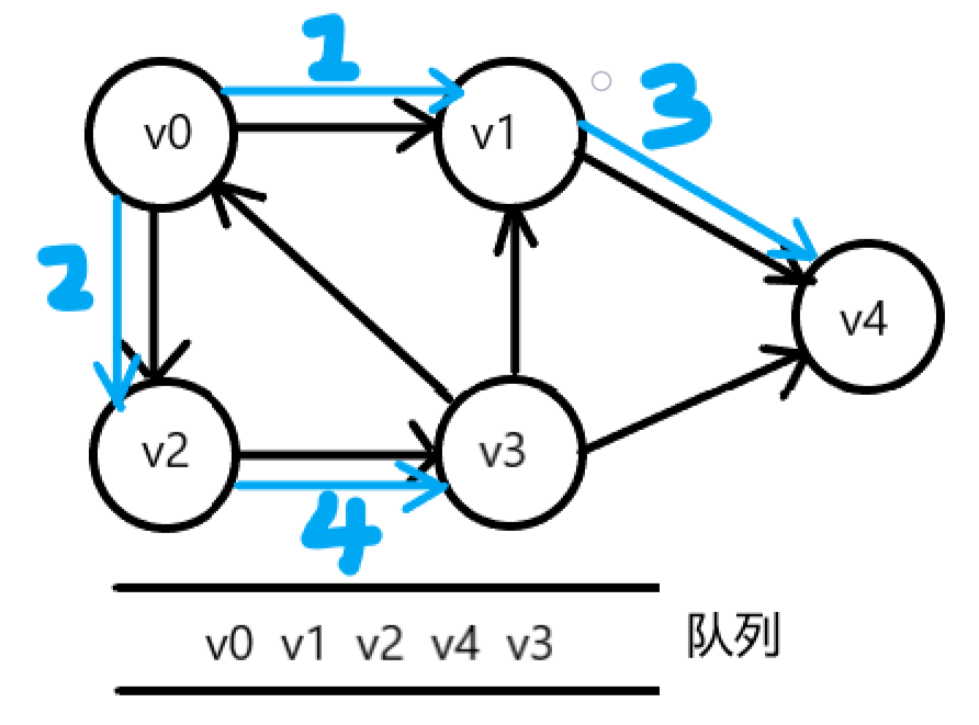
Storage structure of graph
Adjacency matrix adjacency table
adjacency matrix
(array representation)
Use a one-dimensional array to store the vertices in the graph
A two-dimensional array is used to store the edges (adjacency relationship between vertices) = adjacency matrix
n vertices, the square matrix of nxn when adjacent matrix.


The adjacency matrix of an undirected graph must be a symmetric matrix.
1. For an undirected graph, the degree of vertex i = the number of non-zero elements in row I of the adjacency matrix.
For a directed graph, the degree of the vertex i = the number of non-zero elements in row I of the adjacency matrix
Penetration = number of non-zero elements in column i of adjacency matrix
2. To judge whether two vertices have edges, just test whether the corresponding position element in the adjacency matrix is 1
3. Find all adjacent points of vertex i, scan row I of the adjacency matrix, and find the adjacent points if there are non-0 elements.
#include<iostream>
using namespace std;
const int MaxSize = 10;  //Maximum number of vertices in the graph
int visited[MaxSize] = { 0 };  //visited initialization
template <typename T>
class MGragh
{
	T vertex[MaxSize]; //An array of vertices
	int edge[MaxSize][MaxSize];  //An array of edges
	int vertexNum, edgeNum;  //Number of vertices and edges
public:
	MGragh(T a[], int n, int e);//Constructor
	~MGragh() { }; //Destructor, adjacency matrix is static storage, non configuration, and will be released automatically
	void DFTraverse(int v);//Depth first
	void BFTraverse(int v);//Breadth first
};
template<typename T>
MGragh<T>::MGragh(T a[], int n, int e)
{
	int i, j, k;
	vertexNum = n;
	edgeNum = e;
	for (int i = 0; i < vertexNum; i++)  //Store vertices
		vertex[i] = a[i];
	for (i = 0; i < vertexNum; i++)  //Initialize adjacency matrix
		for (j = 0; j < vertexNum; j++)
			edge[i][j] = 0;
	for (k = 0; k < edgeNum; k++)  //Enter each edge in turn
	{
		cout << "Please enter page" << k + 1 << "Strip edge";
		cin >> i >> j;
		edge[i][j] = 1;  //Here is the creation of undirected graph
		edge[j][i] = 1;
	}
}
template <typename T>
void MGragh<T>::DFTraverse(int v)  //Depth first traversal
{
	cout << vertex[v];
	visited[v] = 1;
	for (int j = 0; j < vertexNum; j++)
	{
		if (edge[v][j] == 1 && visited[j] == 0)
			DFTraverse(j);
	}
}
template <typename T>
void MGragh<T>::BFTraverse(int v)  //breadth-first search
{
	int w, j, Q[MaxSize];
	int front = -1;
	int rear = -1;
	cout << vertex[v];

	visited[v] = 1;
	Q[++rear] = v;
	while (front != rear)
	{
		w = Q[++front];
		for (j = 0; j < vertexNum; j++)
		{
			if (edge[w][j] == 1 && visited[j] == 0)
			{
				cout << vertex[j];
				visited[j] = 1;
				Q[++rear] = j;
			}
		}
	}
}
int main()
{
	int i;
	char ch[] = { 'A','B','C','D','E' };
	MGragh<char>MG(ch, 5, 6);
	for (i = 0; i < MaxSize; i++)
		visited[i] = 0;
	cout << "Depth first traversal sequence:";
	MG.DFTraverse(0);
	for (i = 0; i < MaxSize; i++)
		visited[i] = 0;
	cout << "\n Breadth first traversal sequence:";
	MG.BFTraverse(0);

	return 0;
}
Adjacency table
Sequential storage + linked storage.
A child representation similar to a tree.
Edge table: for each vertex v, chain all adjacent points of V into a single chain table.
It is convenient for the head pointers of all side tables to access and operate, and sequential storage is adopted.
Vertex table: the header pointer storing edges and the array storing vertices form the header array of the adjacent table.
There are two kinds of node structures in adjacency table: vertex table node and edge table node
For the network graph, the edge table node adds an info field to store the information on the edge.


#include<iostream>
using namespace std;
const int MaxSize = 10;
int visited[MaxSize] = { 0 };
struct EdgeNode  //Edge table node
{
	int adjvex;  //Adjacency point domain
	EdgeNode* next;
};
template<typename T>
struct VertexNode  //Vertex table node
{
	T vertex;
	EdgeNode* firstEdge;
};
template<typename T>
class ALGraph
{
	VertexNode<T>adjlist[MaxSize];  //An array of vertex tables
	int vertexNum, edgeNum;  //The number of vertices and edges of a graph
public:
	ALGraph(T a[], int n, int e);  //Establish a graph with n vertices and e edges
	~ALGraph(); //Destructor
	void DFTraverse(int v);
	void BFTraverse(int v);
};
template<typename T>
ALGraph<T>::ALGraph(T a[], int n, int e)
{

	EdgeNode* s = nullptr;
	vertexNum = n;
	edgeNum = e;
	for (int i = 0; i < vertexNum; i++)  //initialization
	{
		adjlist[i].vertex = a[i];
		adjlist[i].firstEdge = nullptr;
	}
	for (int i = 0; i < edgeNum; i++)
	{
		cout << "Enter the number of the two vertices to which the edge is attached:";
		int j, k;
		cin >> j >> k;
		s = new EdgeNode;  //Production side table node s
		s->adjvex = k;
		s->next = adjlist[j].firstEdge;  //Insert node s into header
		adjlist[j].firstEdge = s;
	}
}
template<typename T>
ALGraph<T>::~ALGraph()
{
	EdgeNode* p = nullptr, * q = nullptr;
	for (int i = 0; i < vertexNum; i++)
	{
		p = q = adjlist[i].firstEdge;
		while (p != nullptr)
		{
			p = p->next;
			delete q;
			q = p;
		}
	}
}
template<typename T>
void ALGraph<T>::DFTraverse(int v)
{
	int j;
	EdgeNode* p = nullptr;
	cout << adjlist[v].vertex;
	visited[v] = 1;
	p = adjlist[v].firstEdge;
	while (p!=nullptr)
	{
		j = p->adjvex;
		if (visited[j] == 0)
			DFTraverse(j);
		p = p->next;
	}
}
template<typename T>
void ALGraph<T>::BFTraverse(int v)
{
	int w, j, Q[MaxSize];  //Adopt sequential queue
	int front = -1, rear = -1;
	EdgeNode* p = nullptr;
	cout << adjlist[v].vertex;
	visited[v] = 1;
	Q[++rear] = v;
	while (front != rear)
	{
		w = Q[++front];
		p = adjlist[w].firstEdge;
		while (p != nullptr)
		{
			j = p->adjvex;
			if (visited[j] == 0)
			{
				cout << adjlist[j].vertex;
				visited[j] = 1;
				Q[++rear] = j;
			}
			p = p->next;
		}
	}
}
int main()
{
	char ch[] = "ABCDEF";
	ALGraph<char>ALG(ch,5,6);
	for (int i = 0; i < MaxSize; i++)
		visited[i] = 0;
	cout << "The sequence of depth first traversal is:";
	ALG.DFTraverse(0);
	for (int i = 0; i < MaxSize; i++)
		visited[i] = 0;
	cout << "The sequence of breadth first traversal is:";
	ALG.BFTraverse(0);
	//ALG.TopSort();
	return 0;
}
Adjacency matrix vs adjacency table
1. Space performance comparison
Adjacency matrix space cost O(n2), adjacency table space cost O(n+e).
The adjacency matrix stores all possible edges, and the adjacency table only stores the edges that actually appear in the graph.
Adjacency matrices do not require the structural overhead of pointers.
The denser the graph, the higher the spatial efficiency of the adjacency matrix.
2. Time performance comparison
Access all adjacency points of a vertex:
Adjacency matrix O(e/n)
Adjacency table O(n)
3. Uniqueness comparison
Adjacency matrix representation is unique;
The adjacency table representation is not unique, which depends on the input order of edges and the insertion algorithm of nodes in the edge table.
4. Correspondence
The edge table of vertex i in the adjacency table corresponds to row I of the adjacency matrix.
The whole adjacency table can be regarded as the linked storage with row pointer of adjacency matrix.
minimum spanning tree
Spanning tree of connected graph: a minimal connected subgraph containing all vertices in the graph.
A spanning tree with n vertices has only n-1 edges.
Minimum spanning tree: the spanning tree with the lowest cost.
Prim algorithm
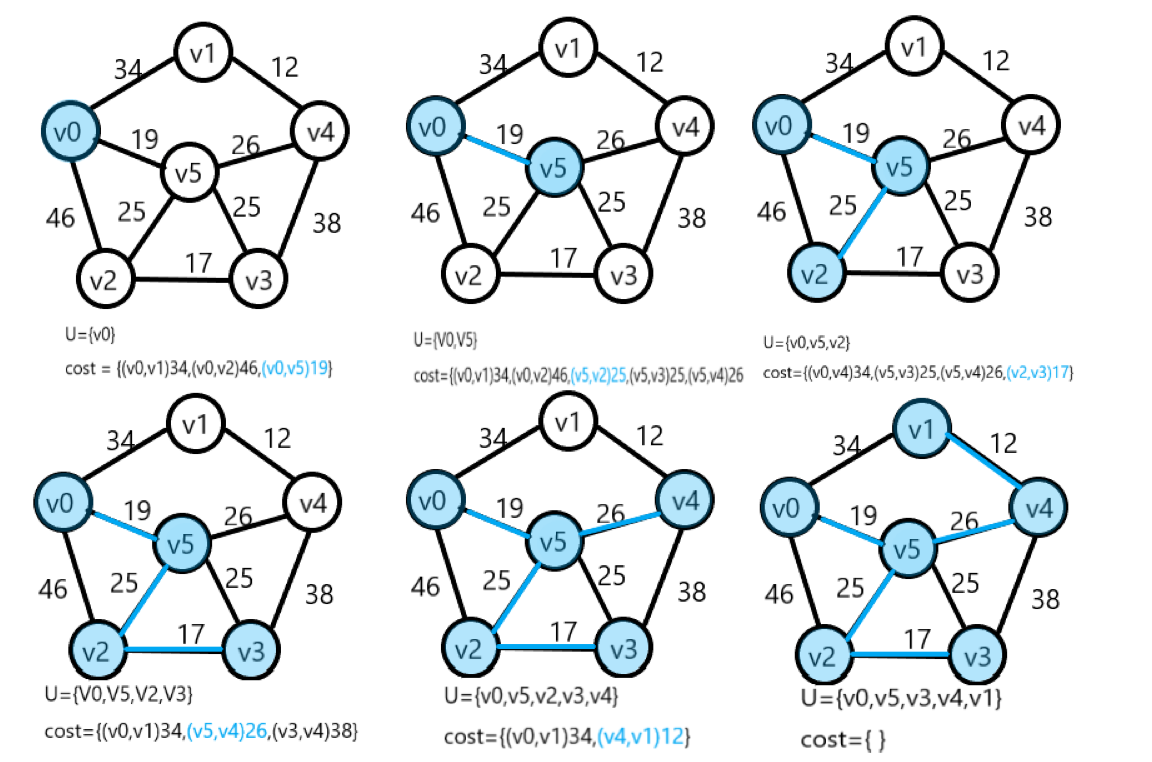
Time complexity: O(n2), independent of the number of edges in the network, suitable for finding the minimum spanning tree in dense networks.
Kruskal algorithm
Or the picture above
No loop! If the shortest edge is added to generate a circuit, it is discarded
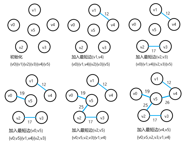
Kruskal algorithm operates based on edges and can be stored in edge set array.
The set where the vertices of connected components are located, because it involves the operations of finding and merging sets, can be realized by merging sets.
Joint search set: organize the elements in the set into the form of a tree.
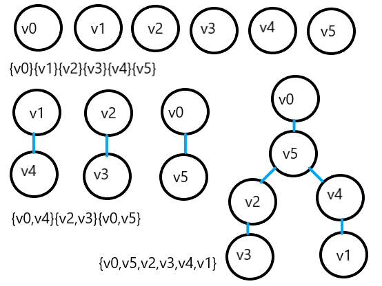
Time complexity: O(elog2e), related to the number of edges, suitable for finding the minimum spanning tree of sparse networks.