Note that we should distinguish between data skew and excessive data. Data skew means that a few tasks are assigned most of the data, so a few tasks run slowly; Excessive data means that the amount of data allocated to all tasks is very large, the difference is not much, and all tasks run slowly.
What is data skew
In short, data skew is that when we calculate data, the dispersion of data is not enough, resulting in a large number of data concentrated on one or several machines. The calculation speed of these data is far lower than the average calculation speed, resulting in the slow calculation process.
When hashing, if there is a large number of values, the hash operation cannot divide the data equally, and can only be processed on one machine, which is data skew.
I believe that most friends who have done data will encounter data skew, which will occur in all links of data development, such as:
- When Hive is used to calculate data, the reduce phase is stuck at 99.99%
- When using SparkStreaming as a real-time algorithm, some executors will always have OOM errors, but the memory utilization of other executors is very low.
A key factor in data skew is the large amount of data, which can reach the level of 100 billion. In fact, the so-called data skew is the uneven distribution of data.
Data skew
Data skew in Hadoop
In Hadoop, the Mapreduce program and Hive program are directly used by users. Although Hive is finally executed by MR (at least at present, Hive memory computing is not popular), the logic of the written content is very different. One is program and the other is Sql, so there is a slight distinction here. The data skew in Hadoop is mainly reflected in the fact that it is stuck at 99.99% in the ruduce stage and can not be ended at 99.99% all the time.
If you look at the log or monitoring interface in detail, you will find:
- One or more reduce is stuck
- Various container s report error OOM
- The amount of data read and written is huge, at least far more than other normal reduce
With the data skew, there will be various strange performances such as the task being kill ed.
Data skew in Spark
Data skew is also common in Spark, including Spark Streaming and Spark Sql. The main manifestations are as follows:
- Error in Executor lost, OOM, Shuffle procedure
- Driver OOM
- A single Executor takes a long time to execute, and the overall task card cannot end at a certain stage
- A working task suddenly fails
In addition, in the spark streaming program, data skew is more likely to occur, especially when the program contains some operations such as sql join and group. Because we generally do not allocate much memory when spark streaming program is running, once some data skew occurs in this process, it is very easy to cause OOM.
Data skew in Hive
The task progress is maintained at 99% (or 100%) for a long time. Check the task monitoring page and find that only a few (1 or several) reduce subtasks have not been completed. Because the amount of data processed is too different from other reduce. The difference between the number of records in a single reduce and the average number of records is too large, usually up to three times or more. The longest duration is greater than the average duration.
Experience: Hive's data skew generally occurs on Group By and Join On in Sql, and is deeply bound to data logic.
Causes of data skew
Why does DateSkew appear in Hive warehouse
The root cause of data skew in the data warehouse is that there are too many values. There are three reasons for the excessive number of job seekers.
Causes:
- Uneven key distribution
- Characteristics of business data
- Null value, a large number of tourist users log in and visit.
- The data types do not match. When using the data imported from mysql data and the data in hive data warehouse for joint query, there may be an int type in mysql and a string type in hive, and the data of these string types will be overstocked together.
- There are problems with the table structure itself. For example, the fields in this region are all cities. Beijing is a value and Taiyuan is a value. At that time, the amount of data in Beijing will be particularly large, resulting in data skew. This example is quite extreme. I just want to say that there are great differences in regional population and data volume.
Why does DateSkew appear in Spark
Reasons for data skew:
The reason for data skew can only be due to the shuffle operation. In the process of shuffle, the problem of data skew occurs. Because the data corresponding to one or some keys is much higher than other keys. Shuffle data leads to uneven data distribution, but the performance of machines at all nodes is the same, and the program is the same, that is, the amount of data is inconsistent, so the execution time of task is determined by the amount of data.
Data partition policy:
- Random partition: the probability of any partition allocated to each data is equal
- Hash partition: use the hash partition value of data,% number of partitions. (causes of data skew)
- Range partition: divide the data range and allocate the data to different ranges (distributed global sorting)
Positioning data skew problem
- Check the operators that will generate shuffle s in the code, such as distinct, groupByKey, reduceByKey, aggregateByKey, join, cogroup, repartition and other operators, and judge whether there will be data skew here according to the code logic.
- Check the log file of Spark job. The log file will record the error to a certain line of code. You can determine the stage in which the error occurs (which stage generates the task is particularly slow) according to the code position to which the exception is located, and locate the corresponding shuffle operator through the stage to determine where the data skew occurs.
To view the distribution of data skew key s:
//Use the sampling operator sample in spark to check the distribution of corresponding key s
val sampledPairs = pairs.sample(false, 0.1)  //sampling
val sampledWordCounts = sampledPairs.countByKey()
sampledWordCounts.foreach(println(_))
Principle of data skew generation
If you are familiar with MapReduce's shuffle process or Spark's shuffle, you don't need to look at this picture at all, because the picture is also casually found by the author and I didn't want to put it here. To add another word, taking MR as an example, it is because the number of data sets is balanced after the shuffle data is grouped by HashPartitioner. The effect of data grouping is roughly as follows:
Operation to generate data skew
| Key operations | situation | result |
|---|---|---|
| Join | One of the tables is small, but the key set | The data distributed to one or several Reduce is much higher than the average |
| Large table and large table, but there are too many 0 values or null values in the judgment field of bucket division | These null values are processed by a redice, which is very slow | |
| group by | The group by dimension is too small, and the quantity of a value is too large | Reducing a value is time consuming |
| Count(DISTINCT XXX) | Too many special values | Reducing this special value is time consuming |
| reduceByKey | There is too much of a value | Reducing a value is time consuming |
| countByKey | There is too much of a value | Reducing a value is time consuming |
| groupByKey | There is too much of a value | Reducing a value is time consuming |
Tilt data processing schemes under different conditions
Processing in Hql and SparkSql
Join
Small table join large table
It is mainly considered to use Map Join instead of Reduce Join.
Use map join to make small dimension tables (the number of records less than 1000) advance into memory. Complete reduce on the map side.
Since the author has previously summarized how to use map join, there is no more statement here. Can refer to hive sql data skew -- how to use map join for large tables and small tables
Large table join large table skewjoin
- When the key has an invalid value:
Change the empty key into a string plus a random number, and divide the tilted data into different reduce. Because the null value is not associated, the final result will not be affected after processing. The treatment method is as follows:
SELECT *
FROM log a
LEFT JOIN bmw_users b
ON CASE WHEN a.user_id IS NULL THEN concat('dp_hive',rand()) >ELSE a.user_id END = b.user_id;
- When all key values are valid
You can use hive to configure:
-- Specifies whether to turn on data skew join Runtime optimization, which is not enabled by default false.
set hive.optimize.skewjoin=true;
-- Judge the threshold of data skew, if join Found the same in key If it exceeds this value, it is considered to be the key Is tilt key. The default is 100000.
-- Generally, it can be set as the total number of records processed/reduce 2 of the number-4 Times.
set hive.skewjoin.key=100000;
-- Specifies whether to turn on data skew join Compile time optimization. It is not enabled by default false.
set hive.optimize.skewjoin.compiletime=true;
Specifically, based on the skewed key stored in the original data, an execution plan will be created separately for the skewed key during compilation, while other keys also have an execution plan to join. Then, perform the union of the two joins generated above. Therefore, unless the same skewed key exists in the two join tables at the same time, the join of the skewed key will be optimized to map side join. In addition, this parameter is similar to hive optimize. The main difference between skewjoins is that this parameter uses the skew information stored in metastore to optimize the execution plan at compile time. If there is no tilt information in the metadata, this parameter is invalid. Generally, both parameters can be set to true. If there is tilt information in the metadata, hive optimize. Sketchjoin does nothing.
data type mismatch
If the data types do not match, you can directly unify the primary keys of the two tables.
select *
from users a
left outer join logs b
on a.usr_id = cast(b.user_id as string)
The associated primary key contains a large number of empty keys
This situation needs to be handled according to the scenario, which is divided into single condition joint query and multi condition joint query. If it is a multi condition joint query, multiple primary keys can be spliced to generate new primary keys to avoid the situation of empty primary keys as much as possible. Of course, this situation needs to be closely combined with business data to ensure that one of multiple related keys in the data is not empty as much as possible. Yes, the number of empty keys can be kept at the normal grouping level, which can also greatly improve the query performance. If we can't guarantee it, we should process each associated primary key in the way of single condition Association. Examples are as follows:
--Data skew SQL
select *
from advertisement_log log
left join user_center user
on log.open_id = user.open_id
and log.union_id = user.union_id

--Adjusted sql
select *
from advertisement_log log
left join user_center user
on concat_ws('_',log.open_id,log.union_id) = concat_ws('_',user.open_id,user.union_id)
For single condition joint query, the following two methods are recommended:
Solution 1: user_ Those whose ID is empty do not participate in association
SELECT *
FROM log a
JOIN bmw_users b
  ON a.user_id IS NOT NULL
 AND a.user_id = b.user_id
UNION ALL
SELECT *
FROM log a
WHERE a.user_id IS NULL;
Solution 2: give null value a new key value
SELECT *
FROM log a
LEFT JOIN bmw_users b
ON CASE WHEN a.user_id IS NULL THEN concat('dp_hive',rand()) ELSE a.user_id END = b.user_id;
Conclusion:
Method 2 is more efficient than method 1, not only io less, but also less homework. Solution 1: the log table is read twice, and jobs is 2. This is suitable for the skew problem caused by optimizing invalid IDS (such as - 99, '', null, etc.). Changing an empty key into a string and adding a random number can divide the skewed data into different reduce to solve the problem of data skew.
The data volume of a few keys in the associated primary key is huge
When the business logic optimization effect is not great, sometimes the inclined data can be taken out and processed separately. Finally, the union went back.
The author encountered this situation when processing the log table data, mainly the log data of different buried points. The amount of data clicked by hot buried points and cold buried points is very large, with a difference of four or five data levels. The author designs the buried point table dictionary table according to the requirements, divides the buried points according to the level of data volume, join s them respectively, and finally uses union all to merge the data. This processing method requires in-depth analysis of data, but the processing is relatively simple and effective, and the principle is similar to the solution 1 of empty key. Examples are as follows:
Dictionary table:
CREATE EXTERNAL TABLE dim.event_v1`
(
   `event_id` STRING COMMENT 'event ID',
   `describe` STRING COMMENT 'Event (buried point) description',
   `district` STRING COMMENT 'Event area',
   `part` STRING COMMENT 'Part of the event',
   `action` STRING COMMENT 'behavior[click,Exhibition]',
   `work_table` STRING COMMENT 'Use table'
)
STORED AS textfile
LOCATION '/big-data/dim/event_v1';
Solution:
SELECT /*+MAPJOIN(event)*/
   user_id,
   app_id,
   provice,
   city,
   district
FROM fct.log log
JOIN (
     SELECT
     FROM dim.event_1
     WHERE work_table = 'big_event_log'
)event
ON log.event_id = event.event_id
UNION ALL
SELECT /*+MAPJOIN(event)*/
   user_id,
   app_id,
   provice,
   city,
   district
FROM fct.log log
JOIN (
     SELECT
     FROM dim.event_1
     WHERE work_table = 'small_event_log'
)event
ON log.event_id = event.event_id
Join driven table selection and data volume optimization:
- As for the selection of the drive table, the table with the most uniform distribution of join key s is selected as the drive table;
- Do a good job in column clipping and filter operations to achieve the effect that the amount of data becomes relatively small when the two tables are join ed.
left semi join
This join application scenario is mainly used to replace the in in sql to improve performance. It is used in some scenarios of large table join and small table join. If the associated result only needs to retain the field data in the left table and the duplicate data only needs to appear once in the result, then the left semi join can be used to avoid the skew caused by the large number of values of the associated primary key. In subsequent articles, the author will summarize the usage of left semi join.
Join tilt summary
The inclined summary of join is basically what I encounter at present. If I encounter other situations in the future, I will be more careful.
Count(DISTINCT XXX)
When count distinct, the case that the value is null will be handled separately. For example, you can directly filter the rows with null value and add 1 to the final result. If there are other calculations, you need to perform group by. You can first process the records with empty values separately, and then union them with other calculation results.
When you can perform group operation first, perform group operation first. reduce the key first, and then perform count or distinct count operation.
group by
Note: group by is better than distinct group.
Use sum() + group by to replace count(distinct) to complete the calculation.
Increase the number of reuducers
The default is by the parameter hive exec. reducers. bytes. per. Reducer to infer the number of reducers needed. Available via mapred reduce. Tasks control.
tuning
hive.map.aggr=true
--open map end combiner
set hive.map.aggr=true
Open map combiner. Some aggregation operations will be done in the map, which is more efficient, but requires more memory.
If each piece of data in the map is basically different, aggregation is meaningless. Making a combiner will add to the snake. It is also considerate in hive. Relevant settings can be made through parameters:
hive.groupby.mapaggr.checkinterval = 100000 (default)
hive.map.aggr.hash.min.reduction=0.5(default)
hive.groupby.skewindata=true
--Load balancing on data skew
set hive.groupby.skewindata=true;
First distribute and process randomly, and then distribute and process according to key group by.
When the option is set to true, the generated query plan will have two mrjobs.
- In the first MRJob, the output result set of Map will be randomly distributed to Reduce. Each Reduce will do some aggregation operations and output results. The result of this processing is that the same GroupBy Key may be distributed to different Reduce, so as to achieve the purpose of load balancing;
- The second MRJob is then distributed to Reduce according to the GroupBy Key according to the preprocessed data results (this process can ensure that the same original GroupBy Key is distributed to the same Reduce), and finally complete the final aggregation operation.
It turns the calculation into two mapreduce. In the first one, the keys are randomly marked during the partition of the shuffle process, so that each key is randomly and evenly distributed to each reduce for calculation. However, this can only complete part of the calculation, because the same key is not assigned to the same reduce. Therefore, the second mapreduce is needed. This time, it will return to the normal shuffle. However, the problem of uneven data distribution has been greatly improved in the first mapreduce, so the data skew is basically solved. Because a large number of calculations have been randomly distributed to each node in the first mr.
Increase parallelism
- Scenario: two large tables with uniform data distribution. In order to improve efficiency, mapjoin is used and the method of splitting large tables is adopted.
- Methods: the large table was divided into small tables, and then connected.
Original test form
+----------+------------+
| test.id  | test.name  |
+----------+------------+
| 1        | aa         |
| 2        | bb         |
| 3        | cc         |
| 4        | dd         |
+----------+------------+
Divide it into two parts:
 select * from test tablesample(bucket 1 out of 2 on id);

+----------+------------+
| test.id  | test.name  |
+----------+------------+
| 2        | bb         |
| 4        | dd         |
+----------+------------+
 select * from test tablesample(bucket 2 out of 2 on id);

+----------+------------+
| test.id  | test.name  |
+----------+------------+
| 1        | aa         |
| 3        | cc         |
+----------+------------+
It is divided into four parts:
select * from test tablesample(bucket 1 out of 4 on id);

+----------+------------+
| test.id  | test.name  |
+----------+------------+
| 4        | dd         |
+----------+------------+
select * from test tablesample(bucket 2 out of 4 on id);
+----------+------------+
| test.id  | test.name  |
+----------+------------+
| 1        | aa         |
+----------+------------+
select * from test tablesample(bucket 3 out of 4 on id);

+----------+------------+
| test.id  | test.name  |
+----------+------------+
| 2        | bb         |
+----------+------------+
select * from test tablesample(bucket 4 out of 4 on id);
+----------+------------+
| test.id  | test.name  |
+----------+------------+
| 3        | cc         |
+----------+------------+
tablesample(bucket 3 out of 4 on id), where tablesample is the keyword, bucket keyword, 3 is the sub table to be split, 4 is the number of split tables, and id is the split basis.
*Multi table union all will be optimized into one job
The promotion effect table should be associated with the commodity table. The auction id column in the effect table has both commodity id and digital id, which is associated with the commodity table to obtain the commodity information.
SELECT *
FROM effect a
JOIN (
      SELECT auction_id AS auction_id
      FROM auctions
      UNION ALL
      SELECT auction_string_id AS auction_id
      FROM auctions
     ) b
ON a.auction_id = b.auction_id;
This is better than filtering digital id and string id respectively, and then associating them with the commodity table respectively. Benefits of writing this way: for one MR operation, the commodity table is read only once, and the promotion effect table is read only once. If you change this sql into MR code, when you map, label the record of table a with label A. each time you read a record of the commodity table, label it with label t, and it becomes two < key, value > pairs, < t, digital id, value >, < t, string id, value >. Therefore, the HDFS (Hadoop Distributed File System) reading of the commodity table will only be once.
Eliminate group by in subquery
Original writing:
SELECT *
FROM (
     SELECT *
     FROM t1
     GROUP BY c1, c2, c3
     UNION ALL
     SELECT *
     FROM t2
     GROUP BY c1, c2, c3
     ) t3
GROUP BY c1, c2, c3;
Optimized writing:
SELECT *
FROM (
      SELECT *
      FROM t1
      UNION ALL
      SELECT *
      FROM t2
     ) t3
GROUP BY c1, c2, c3;
In terms of business logic, the group by function in the sub query is the same as that in the outer layer, unless there is a count(distinct) in the sub query. After testing, there is no hive bug of union all, and the data is consistent. The number of MR Jobs is reduced from 3 to 1. t1 is equivalent to a directory and t2 is equivalent to a directory. For map reduce program, t1 and t2 can be used as mutli inputs of map reduce job. This can be solved through a map reduce. Hadoop's computing framework is not afraid of too much data and too many jobs.
Eliminate count(distinct),max, min in subquery
Original writing:
SELECT c1, c2, c3, sum(pv)
FROM (
    SELECT c1, c2, c3, COUNT(c4)
    FROM t1
    GROUP BY c1, c2, c3
    UNION ALL
    SELECT c1, c2, c3, COUNT(DISTINCT c4)
    FROM t2
    GROUP BY c1, c2, c3
) t3
GROUP BY c1, c2, c3;
In this case, we can't directly use union group by, because one of the table operations uses de duplication. In this case, we can eliminate this data skew problem by creating a temporary table.
Optimized writing:
INSERT INTO t4
SELECT c1, c2, c3, COUNT(DISTINCT c4)
FROM t2
GROUP BY c1, c2, c3;

SELECT c1, c2, c3, SUM(pv)
FROM (
    SELECT c1, c2, c3, COUNT(c4)
    FROM t1
    UNION ALL
    SELECT *
    FROM t4
) t3
GROUP BY c1, c2, c3;
reduce takes too long
Assuming that there are a lot of data in the log corresponding to a memberid, the final merging is also very time-consuming. Therefore, we need to find a method to solve the problem of uneven distribution of reduce.
resolvent:
SELECT *
FROM log a
LEFT JOIN (
           SELECT memberid, number
           FROM users d
           JOIN num e
        ) b
ON a.memberid = b.memberid
AND mod(a.pvtime, 30) + 1 = b.number;
Explain that the above num is a table with one column and 30 rows, corresponding to positive integers of 1-30. Expand the users table into N copies (make an appropriate choice based on the tilt degree), and then divide the log data into different reduce according to memberid and pvtime, so as to ensure that the data allocated to each reduce can be relatively uniform.
Too many where conditions
Sometimes, we write too many where conditions to restrict the query. In fact, this is very inefficient. The main reason is that the and condition hive generates an operator with many nested levels when generating the execution plan.
- Solution:
1) Write the value corresponding to the filter criteria into a small table, and then join to the main table at one time;
2) Or write a udf (user-defined function), read these preset values, and use udf to complete this and data filtering operation.
There are many grouping results, but you only need topK
Original writing:
SELECT mid, url, COUNT(1) AS cnt
FROM (
      SELECT *
      FROM r_atpanel_log
      WHERE pt = '20190610'
      AND pagetype = 'normal'
    ) subq
GROUP BY mid, url
ORDER BY cnt DESC
LIMIT 15;
Optimized writing:
SELECT *
FROM (
      SELECT mid, url, COUNT(1) AS cnt
      FROM (
            SELECT *
            FROM r_atpanel_log
            WHERE pt = '20190610'
            AND pagetype = 'normal'
          ) subq
      GROUP BY mid, url
) subq2
WHERE cnt > 100
ORDER BY cnt DESC
LIMIT 15;
It can be seen that we first filter out irrelevant content and then sort it, which is much faster.
Specific methods for Spark to solve data skew
Solution 1: use Hive ETL to preprocess data
Scenario:
It is Hive table that causes data skew. If the data in the Hive table itself is very uneven (for example, a key corresponds to 1 million data, and other keys correspond to 10 data), and the business scenario requires frequent use of Spark to perform an analysis operation on the Hive table, this technical scheme is more suitable.
Scheme realization idea:
At this time, you can evaluate whether data preprocessing can be performed through Hive (that is, aggregate the data according to the key through Hive ETL in advance, or join with other tables in advance), and then the data source in Spark job is not the original Hive table, but the preprocessed Hive table. At this time, since the data has been aggregated or joined in advance, it is not necessary to use the original shuffle operator to perform such operations in Spark jobs.
Scheme implementation principle:
This solution solves the problem of data skew from the root, because it completely avoids the implementation of shuffle operators in spark, so there will certainly be no problem of data skew. However, we should also remind you that this method is a temporary solution rather than a permanent solution. After all, the data itself has the problem of uneven distribution, so when shuffling operations such as group by or join are performed in Hive ETL, there will still be data skew, resulting in very slow speed of Hive ETL. We just advance the occurrence of data skew to Hive ETL to avoid data skew in Spark Program.
Advantages of the scheme:
The implementation is simple and convenient, and the effect is very good. The data skew is completely avoided, and the performance of Spark operation will be greatly improved.
Disadvantages of the scheme:
Treat symptoms but not root causes, data skew will still occur in Hive ETL.
Practical experience of the scheme:
In some projects where Java systems are combined with Spark, there will be scenes where java code frequently calls Spark jobs, and the execution performance of Spark jobs is very high, so this scheme is more suitable. The Hive ETL that tilts the data to the upstream only executes once a day, which is relatively slow. After that, when Java calls Spark job, the execution speed will be very fast, which can provide a better user experience.
Project experience:
This scheme is used in an Internet interactive user behavior analysis system. The system mainly allows users to submit data analysis and statistics tasks through Java Web system, and the back end submits spark jobs through Java for data analysis and statistics. Spark operation speed must be fast and within 10 minutes as far as possible, otherwise the speed is too slow and the user experience will be very poor. Therefore, we advance the shuffle operation of some spark jobs to Hive ETL, so that spark can directly use the preprocessed Hive intermediate table, reduce the shuffle operation of spark as much as possible, greatly improve the performance, and improve the performance of some jobs by more than 6 times.
Solution 2: filter a few key s that cause skew
Scenario:
If it is found that there are only a few keys that cause skew and have little impact on the calculation itself, this scheme is very suitable. For example, 99% of keys correspond to 10 pieces of data, but only one key corresponds to 1 million data, resulting in data skew.
Scheme realization idea:
If we judge that the few keys with a large amount of data are not particularly important to the execution and calculation results of the job, we can simply filter out the few keys directly. For example, in Spark SQL, you can use the where clause to filter out these keys, or execute the filter operator on RDD in Spark Core to filter out these keys. If you need to dynamically determine which key has the largest amount of data each time the job is executed, and then filter it, you can use the sample operator to sample the RDD, calculate the number of each key, and filter out the key with the largest amount of data.
Scheme implementation principle:
After filtering out the keys that cause data skew, these keys will not participate in the calculation. Naturally, it is impossible to generate data skew.
Advantages of the scheme:
The implementation is simple, and the effect is also very good. It can completely avoid data skew.
Disadvantages of the scheme:
There are few applicable scenarios. In most cases, there are still many key s leading to tilt, not only a few.
Practical experience of the scheme:
In the project, we have also adopted this solution to solve data skew. Once, it was found that the Spark job suddenly went OOM when it was running one day. After tracing, it was found that the data of a key in the Hive table was abnormal that day, resulting in a sharp increase in the amount of data. Therefore, it is necessary to sample before each execution, calculate the keys with the largest amount of data in the sample, and then filter those keys directly in the program.
Solution 3: improve the parallelism of shuffle operation
Scenario:
If we have to face the difficulties of data skew, it is recommended to give priority to this scheme, because it is the simplest scheme to deal with data skew.
Scheme realization idea:
In many shuffle operators, the parallelism can be directly specified. When executing the shuffle operator on RDD, pass a parameter to the shuffle operator, such as reduceByKey(1000) (note that if the parallelism is greater than the number of executors * the number of executor core s, whichever is smaller), this parameter sets the number of shuffle read tasks when executing this shuffle operator. For shuffle statements in Spark SQL, such as group by and join, you need to set a parameter, Spark SQL. shuffle. Partitions, which represents the parallelism of shuffle read task. The default value is 200, which is a little too small for many scenarios.
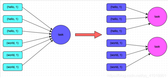
Scheme implementation principle:
Increasing reduce parallelism is actually increasing the number of tasks on the reduce side, so that the amount of data processed by each task is reduced and oom is avoided. That is, by increasing the number of shuffle read tasks, multiple keys originally assigned to one task can be assigned to multiple tasks, so that each task can process less data than the original. For example, if there were originally five keys, each corresponding to 10 pieces of data, and the five keys were assigned to a task, the task would have to process 50 pieces of data. After adding the shuffle read task, each task will be assigned a key, that is, each task will process 10 pieces of data, so the execution time of each task will naturally become shorter. The specific principle is shown in the figure below.
Advantages of the scheme:
The implementation is relatively simple, which can effectively alleviate and mitigate the impact of data skew.
Disadvantages of the scheme:
It only alleviates the data skew and does not completely eradicate the problem. According to practical experience, its effect is limited. The map side keeps writing data, and the reduce task keeps reading data from the specified location. If there are many tasks, the reading speed increases, but the total amount of reduce processing corresponding to each key remains unchanged. Therefore, it does not fundamentally solve the problem of data skew, but tries to reduce the amount of data of the reduce task as much as possible, which is applicable to the problem of large amount of data corresponding to more keys;
Imagine that if only one key has a large amount of data, the high parallelism of other keys is a waste of resources;
Practical experience of the scheme:
This solution usually can not completely solve the data skew, because if there are some extreme cases, such as a key with 1 million data, no matter how many tasks you increase, the key with 1 million data will certainly be allocated to a task for processing, so the data skew is bound to occur. Therefore, this scheme can only be said to be the first means to try to use when finding data skew. It is just trying to use simple methods to alleviate data skew, or it can be used in combination with other schemes.
Solution 4: two-stage aggregation (local aggregation + global aggregation)
Scenario:
This scheme is more applicable when performing aggregate shuffle operators such as reduceByKey on RDD or group by statements in Spark SQL.
Scheme realization idea:
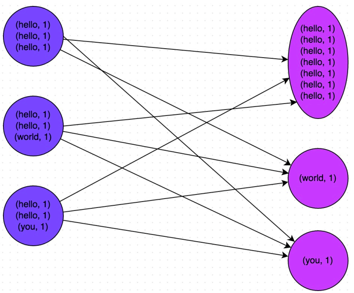
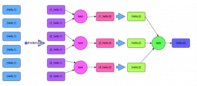
The core implementation idea of this scheme is two-stage aggregation. The first is local aggregation. First, mark each key with a random number, such as a random number within 10. At this time, the original same key will become different. For example, (hello, 1) (hello, 1) (hello, 1) (hello, 1), it will become (1_hello, 1) (1_hello, 1) (2_hello, 1) (2_hello, 1) (2_hello, 1). Then, perform reduceByKey and other aggregation operations on the data marked with random numbers to conduct local aggregation, and the local aggregation result will become (1_hello, 2) (2_hello, 2). Then remove the prefix of each key and it will become (hello,2)(hello,2). Conduct global aggregation again and you can get the final result, such as (hello, 4).
Scheme implementation principle:
By adding a random prefix to the original same key to multiple different keys, the data originally processed by one task can be dispersed to multiple tasks for local aggregation, so as to solve the problem of excessive data processing by a single task. Then remove the random prefix and conduct global aggregation again to get the final result. The specific principle is shown in the figure below.
Advantages of the scheme:
For the data skew caused by the shuffle operation of aggregation class, the effect is very good. Generally, the data skew can be solved, or at least the data skew can be greatly alleviated to improve the performance of Spark jobs by more than several times.
Disadvantages of the scheme:
It is only applicable to the shuffle operation of aggregation class, and the scope of application is relatively narrow. If it is a shuffle operation of the join class, you have to use other solutions.
// The first step is to add a random prefix to each key in the RDD.
JavaPairRDD<String, Long> randomPrefixRdd = rdd.mapToPair(
        new PairFunction<Tuple2<Long,Long>, String, Long>() {
            private static final long serialVersionUID = 1L;
            @Override
            public Tuple2<String, Long> call(Tuple2<Long, Long> tuple)
                    throws Exception {
                Random random = new Random();
                int prefix = random.nextInt(10);
                return new Tuple2<String, Long>(prefix + "_" + tuple._1, tuple._2);
            }
        });

// The second step is to locally aggregate the key s with random prefixes.
JavaPairRDD<String, Long> localAggrRdd = randomPrefixRdd.reduceByKey(
        new Function2<Long, Long, Long>() {
            private static final long serialVersionUID = 1L;
            @Override
            public Long call(Long v1, Long v2) throws Exception {
                return v1 + v2;
            }
        });

// Step 3: remove the random prefix of each key in the RDD.
JavaPairRDD<Long, Long> removedRandomPrefixRdd = localAggrRdd.mapToPair(
        new PairFunction<Tuple2<String,Long>, Long, Long>() {
            private static final long serialVersionUID = 1L;
            @Override
            public Tuple2<Long, Long> call(Tuple2<String, Long> tuple)
                    throws Exception {
                long originalKey = Long.valueOf(tuple._1.split("_")[1]);
                return new Tuple2<Long, Long>(originalKey, tuple._2);
            }
        });

// The fourth step is to aggregate the RDD S without random prefix globally.
JavaPairRDD<Long, Long> globalAggrRdd = removedRandomPrefixRdd.reduceByKey(
        new Function2<Long, Long, Long>() {
            private static final long serialVersionUID = 1L;
            @Override
            public Long call(Long v1, Long v2) throws Exception {
                return v1 + v2;
            }
        });
Solution 5: convert reduce join to map join
Scenario:
When using join operations on RDDS or join statements in Spark SQL, and the amount of data in an RDD or table in the join operation is relatively small (such as hundreds of M or one or two G), this scheme is more applicable.
Scheme realization idea:
Instead of using the join operator for connection operation, the Broadcast variable and map operator are used to realize the join operation, so as to completely avoid the operation of shuffle class and the occurrence and occurrence of data skew. Pull the data in the smaller RDD directly into the memory of the Driver through the collect operator, and then create a Broadcast variable for it; Then execute the map operator on another RDD. In the operator function, obtain the full amount of data of the smaller RDD from the Broadcast variable, and compare it with each data of the current RDD according to the connection key. If the connection key is the same, then connect the data of the two RDDS in the way you need.
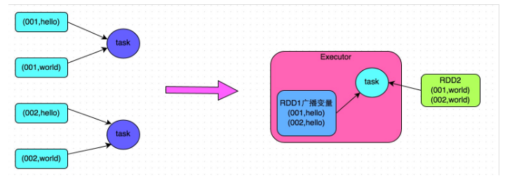
Scheme implementation principle:
Ordinary join will go through the shuffle process. Once shuffled, it is equivalent to pulling the data of the same key into a shuffle read task for join. At this time, it is reduce join. However, if an RDD is relatively small, broadcast small RDD full data + map operator can be used to achieve the same effect as join, that is, map join. At this time, shuffle operation and data skew will not occur. The specific principle is shown in the figure below.
Advantages of the scheme:
The effect of data skew caused by join operation is very good, because shuffle and data skew will not occur at all.
Disadvantages of the scheme:
There are few applicable scenarios, because this scheme is only applicable to one large table and one small table. After all, we need to broadcast the small table. At this time, memory resources will be consumed. A full amount of small RDD data will reside in the memory of driver and each Executor. If the RDD data we broadcast is large, such as more than 10G, memory overflow may occur. Therefore, it is not suitable for the situation that both are large tables.
// First, collect the RDD data with a small amount of data into the Driver.
List<Tuple2<Long, Row>> rdd1Data = rdd1.collect()
// Then use Spark's broadcast function to convert the small RDD data into broadcast variables, so that each Executor has only one RDD data.
// It can save memory space as much as possible and reduce network transmission performance overhead.
final Broadcast<List<Tuple2<Long, Row>>> rdd1DataBroadcast = sc.broadcast(rdd1Data);

// Perform a map class operation on another RDD instead of a join class operation.
JavaPairRDD<String, Tuple2<String, Row>> joinedRdd = rdd2.mapToPair(
        new PairFunction<Tuple2<Long,String>, String, Tuple2<String, Row>>() {
            private static final long serialVersionUID = 1L;
            @Override
            public Tuple2<String, Tuple2<String, Row>> call(Tuple2<Long, String> tuple)
                    throws Exception {
                // In the operator function, the rdd1 data in the local Executor is obtained by broadcasting variables.
                List<Tuple2<Long, Row>> rdd1Data = rdd1DataBroadcast.value();
                // The data of rdd1 can be converted into a Map to facilitate the join operation later.
                Map<Long, Row> rdd1DataMap = new HashMap<Long, Row>();
                for(Tuple2<Long, Row> data : rdd1Data) {
                    rdd1DataMap.put(data._1, data._2);
                }
                // Get the key and value of the current RDD data.
                String key = tuple._1;
                String value = tuple._2;
                // From the rdd1 data Map, obtain the data that can be join ed according to the key.
                Row rdd1Value = rdd1DataMap.get(key);
                return new Tuple2<String, String>(key, new Tuple2<String, Row>(value, rdd1Value));
            }
        });

// Here's a hint.
// The above method is only applicable to the key in rdd1. There is no repetition. All of them are unique scenarios.
// If there are multiple identical key s in rdd1, you have to use the operation of flatMap class. You can't use map when joining, but you have to traverse all the data in rdd1 for joining.
// Each data in rdd2 may return multiple join ed data.
Solution 6: sample samples the tilt key and splits the join operation
This method is different from the processing method of multiple values of the same key in sql.
Scenario:
When join ing two RDD/Hive tables, if the data volume is large and "solution 5" cannot be adopted, then you can take a look at the key distribution in the two RDD/Hive tables. If data skew occurs because the data volume of a few keys in one RDD/Hive table is too large, and all keys in the other RDD/Hive table are evenly distributed, this solution is more appropriate.
Scheme realization idea:
For the RDD containing a few key s with too much data,
- A sample is sampled by the sample operator,
- Then count the number of each key and calculate which keys have the largest amount of data.
- Then, the data corresponding to these keys is split from the original RDD to form a separate RDD, and each key is prefixed with a random number within n, which will not cause most of the inclined keys to form another RDD.
- Then, filter out the data corresponding to those inclined keys from another RDD that needs to be join ed and form a separate RDD. Expand each data into n pieces of data. These n pieces of data are sequentially prefixed with a 0~n prefix, which will not cause most inclined keys to form another RDD.
- Then join the independent RDD with random prefix and another independent RDD with n times expansion. At this time, the original same key can be broken into n parts and dispersed into multiple task s for joining. The other two ordinary RDDS can join as usual.
- Finally, the results of the two joins can be combined by using the union operator, which is the final join result.
Scheme implementation principle:
For the data skew caused by join, if only a few keys cause the skew, you can split a few keys into independent RDD S and add random prefixes to break them into n copies for join. At this time, the data corresponding to these keys will not be concentrated on a few tasks, but will be scattered to multiple tasks for join. The specific principle is shown in the figure below.
Advantages of the scheme:
For the data skew caused by join, if only a few keys cause the skew, this method can be used to break up the keys in the most effective way for join. Moreover, only the data corresponding to a few tilt keys need to be expanded n times, and there is no need to expand the full amount of data. Avoid taking up too much memory.
Disadvantages of the scheme:
If there are too many keys leading to skew, for example, thousands of keys lead to data skew, this method is not suitable.
// First, sample 10% of the sample data from rdd1, which contains a few key s that cause data skew.
JavaPairRDD<Long, String> sampledRDD = rdd1.sample(false, 0.1);

// For the sample data RDD, count the occurrence times of each key and sort it in descending order.
// For the data sorted in descending order, take out the data of top 1 or top 100, that is, the first n data with the most key s.
// The specific number of key s with the largest amount of data is up to you to decide. Let's take one as a demonstration.
JavaPairRDD<Long, Long> mappedSampledRDD = sampledRDD.mapToPair(
        new PairFunction<Tuple2<Long,String>, Long, Long>() {
            private static final long serialVersionUID = 1L;
            @Override
            public Tuple2<Long, Long> call(Tuple2<Long, String> tuple)
                    throws Exception {
                return new Tuple2<Long, Long>(tuple._1, 1L);
            }
        });
JavaPairRDD<Long, Long> countedSampledRDD = mappedSampledRDD.reduceByKey(
        new Function2<Long, Long, Long>() {
            private static final long serialVersionUID = 1L;
            @Override
            public Long call(Long v1, Long v2) throws Exception {
                return v1 + v2;
            }
        });
JavaPairRDD<Long, Long> reversedSampledRDD = countedSampledRDD.mapToPair(
        new PairFunction<Tuple2<Long,Long>, Long, Long>() {
            private static final long serialVersionUID = 1L;
            @Override
            public Tuple2<Long, Long> call(Tuple2<Long, Long> tuple)
                    throws Exception {
                return new Tuple2<Long, Long>(tuple._2, tuple._1);
            }
        });
final Long skewedUserid = reversedSampledRDD.sortByKey(false).take(1).get(0)._2;

// Separate the key that causes data skew from rdd1 to form an independent RDD.
JavaPairRDD<Long, String> skewedRDD = rdd1.filter(
        new Function<Tuple2<Long,String>, Boolean>() {
            private static final long serialVersionUID = 1L;
            @Override
            public Boolean call(Tuple2<Long, String> tuple) throws Exception {
                return tuple._1.equals(skewedUserid);
            }
        });
// Ordinary key s that do not cause data skew are separated from rdd1 to form an independent RDD.
JavaPairRDD<Long, String> commonRDD = rdd1.filter(
        new Function<Tuple2<Long,String>, Boolean>() {
            private static final long serialVersionUID = 1L;
            @Override
            public Boolean call(Tuple2<Long, String> tuple) throws Exception {
                return !tuple._1.equals(skewedUserid);
            }
        });

// rdd2 is the rdd with relatively uniform distribution of all key s.
// Here, the data corresponding to the previously obtained key in rdd2 is filtered out and divided into separate RDDS, and the data in RDD is expanded by 100 times using flatMap operator.
// Each data of the expansion is prefixed with 0 ~ 100.
JavaPairRDD<String, Row> skewedRdd2 = rdd2.filter(
         new Function<Tuple2<Long,Row>, Boolean>() {
            private static final long serialVersionUID = 1L;
            @Override
            public Boolean call(Tuple2<Long, Row> tuple) throws Exception {
                return tuple._1.equals(skewedUserid);
            }
        }).flatMapToPair(new PairFlatMapFunction<Tuple2<Long,Row>, String, Row>() {
            private static final long serialVersionUID = 1L;
            @Override
            public Iterable<Tuple2<String, Row>> call(
                    Tuple2<Long, Row> tuple) throws Exception {
                Random random = new Random();
                List<Tuple2<String, Row>> list = new ArrayList<Tuple2<String, Row>>();
                for(int i = 0; i < 100; i++) {
                    list.add(new Tuple2<String, Row>(i + "_" + tuple._1, tuple._2));
                }
                return list;
            }

        });

// Separate the independent RDD of the tilted key separated from rdd1, and each data is prefixed with a random prefix within 100.
// Then join the independent RDD separated from rdd1 with the independent RDD separated from rdd2 above.
JavaPairRDD<Long, Tuple2<String, Row>> joinedRDD1 = skewedRDD.mapToPair(
        new PairFunction<Tuple2<Long,String>, String, String>() {
            private static final long serialVersionUID = 1L;
            @Override
            public Tuple2<String, String> call(Tuple2<Long, String> tuple)
                    throws Exception {
                Random random = new Random();
                int prefix = random.nextInt(100);
                return new Tuple2<String, String>(prefix + "_" + tuple._1, tuple._2);
            }
        })
        .join(skewedUserid2infoRDD)
        .mapToPair(new PairFunction<Tuple2<String,Tuple2<String,Row>>, Long, Tuple2<String, Row>>() {
                        private static final long serialVersionUID = 1L;
                        @Override
                        public Tuple2<Long, Tuple2<String, Row>> call(
                            Tuple2<String, Tuple2<String, Row>> tuple)
                            throws Exception {
                            long key = Long.valueOf(tuple._1.split("_")[1]);
                            return new Tuple2<Long, Tuple2<String, Row>>(key, tuple._2);
                        }
                    });

// Separate RDDS containing ordinary key s from rdd1 and directly join with rdd2.
JavaPairRDD<Long, Tuple2<String, Row>> joinedRDD2 = commonRDD.join(rdd2);

// Combine the result after tilting the key join with the result after ordinary key join and uinon.
// This is the final join result.
JavaPairRDD<Long, Tuple2<String, Row>> joinedRDD = joinedRDD1.union(joinedRDD2);
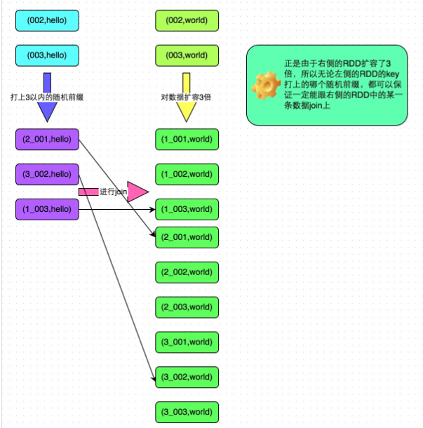
Solution 7: join using random prefix and capacity expansion RDD
Scenario:
If a large number of keys in the RDD cause data skew during the join operation, it is meaningless to split the keys. At this time, the last solution can only be used to solve the problem.
Scheme realization idea:
The implementation idea of this scheme is basically similar to that of "solution 6",
- First, check the data distribution in the RDD/Hive table and find the RDD/Hive table that causes data skew. For example, multiple key s correspond to more than 10000 pieces of data.
- Then, each data of the RDD is prefixed with a random prefix within n.
- At the same time, the capacity of another normal RDD is expanded, and each data is expanded into N data. Each data expanded is prefixed with 0~n in turn.
- Finally, join the two processed RDD S.
Scheme implementation principle:
Change the same key into different keys by adding a random prefix, and then these processed "different keys" can be dispersed into multiple tasks for processing, rather than allowing one task to process a large number of the same keys. The difference between this scheme and "solution 6" is that the previous scheme is to perform special processing on the data corresponding to a few tilt keys as far as possible. Because the processing process needs to expand RDD, the memory occupied by the previous scheme after expanding RDD is not large; This scheme is aimed at the situation that there are a large number of inclined keys. It is impossible to separate some keys for separate processing. Therefore, it can only expand the data capacity of the whole RDD, which requires high memory resources.
Advantages of the scheme:
Basically, the join type data skew can be processed, and the effect is relatively significant. The performance improvement effect is very good.
Disadvantages of the scheme:
This scheme is more to alleviate data skew than to completely avoid data skew. Moreover, the entire RDD needs to be expanded, which requires high memory resources.
Practical experience of the scheme:
When developing a data requirement, I found that a join led to data skew. Before optimization, the execution time of the job is about 60 minutes; After optimization with this scheme, the execution time is shortened to about 10 minutes and the performance is improved by 6 times.
// Firstly, one of the RDD S with relatively uniform key distribution is expanded by 100 times.
JavaPairRDD<String, Row> expandedRDD = rdd1.flatMapToPair(
        new PairFlatMapFunction<Tuple2<Long,Row>, String, Row>() {
            private static final long serialVersionUID = 1L;
            @Override
            public Iterable<Tuple2<String, Row>> call(Tuple2<Long, Row> tuple)
                    throws Exception {
                List<Tuple2<String, Row>> list = new ArrayList<Tuple2<String, Row>>();
                for(int i = 0; i < 100; i++) {
                    list.add(new Tuple2<String, Row>(0 + "_" + tuple._1, tuple._2));
                }
                return list;
            }
        });

// Secondly, another RDD with data tilt key is marked with a random prefix within 100.
JavaPairRDD<String, String> mappedRDD = rdd2.mapToPair(
        new PairFunction<Tuple2<Long,String>, String, String>() {
            private static final long serialVersionUID = 1L;
            @Override
            public Tuple2<String, String> call(Tuple2<Long, String> tuple)
                    throws Exception {
                Random random = new Random();
                int prefix = random.nextInt(100);
                return new Tuple2<String, String>(prefix + "_" + tuple._1, tuple._2);
            }
        });

// join the two processed RDD S.
JavaPairRDD<String, Tuple2<String, Row>> joinedRDD = mappedRDD.join(expandedRDD);
Solution 8: combination of multiple solutions
In practice, it is found that in many cases, if we only deal with relatively simple data tilt scenarios, we can solve them by using one of the above schemes. However, if you want to deal with a more complex data skew scene, you may need to combine multiple schemes. For example, for Spark jobs with multiple data skew links, we can first use solutions 1 and 2 to preprocess part of the data and filter part of the data to alleviate; Secondly, we can improve the parallelism of some shuffle operations and optimize their performance; Finally, you can choose a scheme to optimize its performance for different aggregation or join operations. After thoroughly understanding the ideas and principles of these schemes, we need to flexibly use a variety of schemes according to different situations in practice to solve our own data skew problem.
Solution 9: repartition
This is also a common method. Its essence is to reduce the amount of data processed by task. It usually occurs before shuffle. Of course, it is also a shuffle operation.
epilogue
The above is the scheme of data skew processing and some situations encountered by the author, which will be updated in the future.