Pandas can handle time series in any field. Using Numpy's datetime64 and timedelta64 types, pandas integrates many functions from other Python libraries, such as Scikits.TimeSeries , and create a lot of new functions for processing time series data.

1, Timing creation

1. Four types of time variables

name	describe	Element type	How to create
Datetimes (point / time)	Describe a specific date or point in time	Timestamp	to_datetime or date_range
Timespans (time period)	A period of time defined by a point in time	Period	Period or period_range
Dateoffsets (relative time difference)	Relative size over time (not related to summer / winter)	Dateoffset	DateOffset
Timedeltas (absolute time difference)	Absolute size over time (related to summer / winter)	Timedelta	to_timedelta or timedelta_range

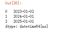
For time Series data, the traditional approach is to represent time components in Series or DataFrame indexes, so that operations can be performed on time elements. However, Series and DataFrame can also directly support time components as data itself. When passed to these constructors, Series and DataFrame extend data type support and functionality for date time, time increment, and period data. However, DateOffset data will be stored as object data.

#Add time component in index, dtype is int64
pd.Series(range(3), index=pd.date_range('2000', freq='D', periods=3))
#Define the time component directly. dtype is datetime64[ns]
pd.Series(pd.date_range('2000', freq='D', periods=3))

2. Creation of time point

Timestamped is the most basic type of time series data that associates values with time points. For pandas objects, this means using point in time.

(a)to_datetime method

Pandas gives a lot of freedom in the input format specification of time point establishment. The following statements can correctly establish the same time point

print(pd.to_datetime('2020.1.1'))
print(pd.to_datetime('2020 1.1'))
print(pd.to_datetime('2020 1 1'))
print(pd.to_datetime('2020 1-1'))
print(pd.to_datetime('2020-1 1'))
print(pd.to_datetime('2020-1-1'))
print(pd.to_datetime('2020/1/1'))
print(pd.to_datetime('1.1.2020'))
print(pd.to_datetime('1.1 2020'))
print(pd.to_datetime('1 1 2020'))
print(pd.to_datetime('1 1-2020'))
print(pd.to_datetime('1-1 2020'))
print(pd.to_datetime('1-1-2020'))
print(pd.to_datetime('1/1/2020'))
print(pd.to_datetime('20200101'))
print(pd.to_datetime('2020.0101'))

#pd.to_datetime('2020\\1\\1') #report errors
#pd.to_datetime('2020`1`1') #report errors
#pd.to_datetime('2020.1 1') #report errors
#pd.to_datetime('1 1.2020') #report errors

Using format parameter to force matching

print(pd.to_datetime('2020\\1\\1',format='%Y\\%m\\%d'))
print(pd.to_datetime('2020`1`1',format='%Y`%m`%d'))
print(pd.to_datetime('2020.1 1',format='%Y.%m %d'))
print(pd.to_datetime('1 1.2020',format='%d %m.%Y'))

You can also use a list to turn it into a point in time index

pd.Series(range(2),index=pd.to_datetime(['2020/1/1','2020/1/2']))

View type

type(pd.to_datetime(['2020/1/1','2020/1/2']))

For DataFrame, if the columns are already in chronological order, use to_datetime can be automatically converted

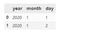
df = pd.DataFrame({'year': [2020, 2020],'month': [1, 1], 'day': [1, 2]})
pd.to_datetime(df)

(b) Time precision and range limitation

The accuracy of Timestamp is far more than day. It can be as small as nanosecond ns, and its range is

pd.to_datetime('2020/1/1 00:00:00.123456789')

#Minimum range
print(pd.Timestamp.min)  #output:Timestamp('1677-09-21 00:12:43.145225')
#Maximum range
print(pd.Timestamp.min)  #output:Timestamp('2262-04-11 23:47:16.854775807')

(c)date_range method

start/end/periods / freq (interval method) is the most important parameter of this method. Given three of them, the remaining one will be sing ed

The freq parameters are as follows:

Symbol	D/B	W	M/Q/Y	BM/BQ/BY	MS/QS/YS	BMS/BQS/BYS	H	T	S
describe	Days / working days	week	end of the month	Month / season / year end	Month / quarter / year end working day	Month / quarter / year beginning date	Time	minute	second

3.Dateoffset object

(a) The difference between DateOffset and Timedelta

The characteristic of the absolute time difference of Timedelta is that whether it is winter time or summer time, the increase or decrease of 1 day is only 24 hours

DateOffset relative time difference means that no matter whether a day is 23 / 24 / 25 hours, the increase or decrease of 1 day is consistent with the same time of the day

For example, in the 03 hours of 2020, 29 hours in the UK, the 01:00:00 clock changed 1 hours to 2020, 03 months 29, 02:00:00, and began daylight saving time.

ts = pd.Timestamp('2020-3-29 01:00:00', tz='Europe/Helsinki')
ts + pd.Timedelta(days=1)

ts = pd.Timestamp('2020-3-29 01:00:00', tz='Europe/Helsinki')
ts + pd.DateOffset(days=1)

The tz attribute can be removed to keep the two consistent.

(b) Increase or decrease for a period of time

pd.Timestamp('2020-01-01') + pd.DateOffset(minutes=20) - pd.DateOffset(weeks=2)

(c) Various common offset objects

pd.Timestamp('2020-01-01') + pd.offsets.Week(2)  #Add two weeks
pd.Timestamp('2020-01-01') + pd.offsets.BQuarterBegin(1)  #Start of business quarter

(d) offset operation of sequence

Using the apply function

pd.Series(pd.offsets.BYearBegin(3).apply(i) for i in pd.date_range('20200101',periods=3,freq='Y'))

Use object addition and subtraction directly

pd.date_range('20200101',periods=3,freq='Y') + pd.offsets.BYearBegin(3)

To customize the offset, you can specify the weekmask and holidays parameters

pd.Series(pd.offsets.CDay(3,weekmask='Wed Fri',holidays='2020010').apply(i)
                                  for i in pd.date_range('20200105',periods=3,freq='D'))

2, Index and attribute of time sequence

1. Index slice

rng = pd.date_range('2020','2021', freq='W')
ts = pd.Series(np.random.randn(len(rng)), index=rng)
ts['2020-01-26':'20200726'].head() #The date is from 01-26 to 07-26, and the character itself is converted to reasonable

Subset index 2

#Take July data only
ts['2020-7'].head()
#Support mixed form index
ts['2011-1':'20200726'].head()

3. Attributes of time points

Information about time can be easily obtained with dt object

#52 weeks in 2020
pd.Series(ts.index).dt.week
#What's the day of the week
pd.Series(ts.index).dt.day

Using strftime to modify time format

pd.Series(ts.index).dt.strftime('%Y-Interval 1-%m-Interval 2-%d').head()

For datetime objects, you can get information directly from the properties

#Month of the week
pd.date_range('2020','2021', freq='W').month
#Month of the week
pd.date_range('2020','2021', freq='W').weekday #The number of the day of the week with Monday=0, Sunday=6

3, Resampling

Resampling refers to the resample function, which can be regarded as the group by function of the sequential version

1. Basic operation of example object

The sampling frequency is generally set to the offset character mentioned above

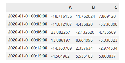
df_r = pd.DataFrame(np.random.randn(1000, 3),index=pd.date_range('1/1/2020', freq='S', periods=1000),
                  columns=['A', 'B', 'C'])
r = df_r.resample('3min')
r.sum()

2. Sample aggregation

df_r = pd.DataFrame(np.random.randn(1000, 3),index=pd.date_range('1/1/2020', freq='S', periods=1000),
                  columns=['A', 'B', 'C'])
r = df_r.resample('3T')

#Only one value is required
r['A'].mean()
#Represents multiple
r['A'].agg([np.sum, np.mean, np.std])
#Using lambda
r.agg({'A': np.sum,'B': lambda x: max(x)-min(x)})

3. Iteration of sampling group

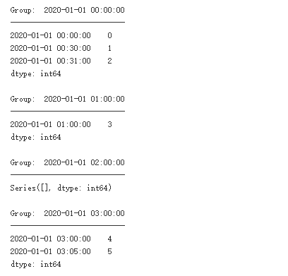
The iteration of sampling group is similar to that of group by, and each group can be operated separately

small = pd.Series(range(6),index=pd.to_datetime(['2020-01-01 00:00:00', '2020-01-01 00:30:00'
                                                 , '2020-01-01 00:31:00','2020-01-01 01:00:00'
                                                 ,'2020-01-01 03:00:00','2020-01-01 03:05:00']))
resampled = small.resample('H')
for name, group in resampled:
    print("Group: ", name)
    print("-" * 27)
    print(group, end="\n\n")

4, Window function

1.Rolling

(a) Common aggregation

s = pd.Series(np.random.randn(1000),index=pd.date_range('1/1/2020', periods=1000))
#
s.rolling(window=50)
#
s.rolling(window=50).mean()
#min_periods is the threshold value of the number of non missing data points needed
s.rolling(window=50,min_periods=3).mean()

In addition, count / sum / mean / median / min / max / STD / var / skew / Kurt / quantity / cov / corr are common aggregate functions

(b) Application aggregation of rolling

When using apply aggregation, just remember that the incoming Series is window size Series, and the output must be scalar,

#Calculate coefficient of variation
s.rolling(window=50,min_periods=3).apply(lambda x:x.std()/x.mean()).head()

(c) Rolling based on time

Select the closed='right '(default) \'left'\'both'\'neither' parameter to determine the endpoint inclusion

s.rolling('15D').mean().head()
#Add closed
s.rolling('15D', closed='right').sum().head()

2.Expanding

(a) expanding function

The common expanding function is equivalent to rolling(window=len(s),min_periods=1) is the cumulative calculation of the sequence, and apply is also applicable

#rolling
s.rolling(window=len(s),min_periods=1).sum().head()
#expanding
s.expanding().sum().head()
#apply
s.expanding().apply(lambda x:sum(x)).head()

(b) Several special Expanding type functions

cumsum/cumprod/cummax/cummin are all special expanding cumulative calculation methods

shift/diff/pct_change refers to element relationship

① shift means that the sequence index does not change, but the value moves backward

② diff refers to the difference between the front and back elements. The period parameter indicates the interval, which is 1 by default and can be negative

③pct_change is the percentage change of elements before and after the value, and the period parameter is similar to diff