- lenet model introduction
- lenet network construction
- Image recognition using lenet - Fashion MNIST dataset
Convolutional Neural Networks
Limitations of using full connection layer:
- The pixels adjacent to an image in the same column may be far apart in this vector. The patterns they form may be difficult to identify by models.
- For large-scale input image, using full connection layer is easy to cause the model to be too large.
Advantages of using convolution:
- The convolution layer retains the input shape.
- The convolution layer repeatedly calculates the same convolution kernel and the input at different positions through the sliding window, so as to avoid the parameter size being too large.
LeNet model
LeNet is divided into convolution layer block and full connection layer block. We will introduce the two modules respectively.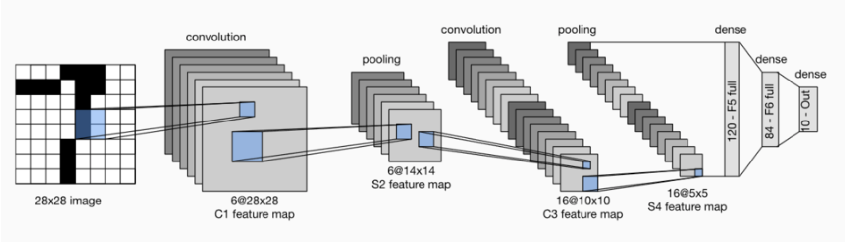
The basic unit in the convolution layer block is the convolution layer followed by the average pooling layer: the convolution layer is used to identify spatial patterns in the image, such as lines and local objects, and the average pooling layer after the convolution layer is used to reduce the sensitivity of the convolution layer to location.
The convolution layer block consists of two such basic units stacked repeatedly. In the convolution layer block, each convolution layer uses the
And use sigmoid to activate the function on the output. The number of output channels of the first convolution layer is 6, and the number of output channels of the second convolution layer is increased to 16.
The full connection layer block includes three full connection layers. Their output numbers are 120, 84 and 10 respectively, where 10 is the number of output categories.
Next, we implement the LeNet model through the Sequential class.
#import
import sys
sys.path.append("/home/kesci/input")
import d2lzh1981 as d2l
import torch
import torch.nn as nn
import torch.optim as optim
import time
#net
class Flatten(torch.nn.Module):  #Flattening operation
    def forward(self, x):
        return x.view(x.shape[0], -1)

class Reshape(torch.nn.Module): #Reshape image size
    def forward(self, x):
        return x.view(-1,1,28,28)      #(B x C x H x W)

net = torch.nn.Sequential(     #Lelet
    Reshape(),
    nn.Conv2d(in_channels=1, out_channels=6, kernel_size=5, padding=2), #b*1*28*28  =>b*6*28*28
    nn.Sigmoid(),
    nn.AvgPool2d(kernel_size=2, stride=2),                              #b*6*28*28  =>b*6*14*14
    nn.Conv2d(in_channels=6, out_channels=16, kernel_size=5),           #b*6*14*14  =>b*16*10*10
    nn.Sigmoid(),
    nn.AvgPool2d(kernel_size=2, stride=2),                              #b*16*10*10  => b*16*5*5
    Flatten(),                                                          #b*16*5*5   => b*400
    nn.Linear(in_features=16*5*5, out_features=120),
    nn.Sigmoid(),
    nn.Linear(120, 84),
    nn.Sigmoid(),
    nn.Linear(84, 10)
)
Next, we construct a single channel data sample with a height of 28 and a width of 28, and perform forward calculation layer by layer to see the output shape of each layer.
#print
X = torch.randn(size=(1,1,28,28), dtype = torch.float32)
for layer in net:
    X = layer(X)
    print(layer.__class__.__name__,'output shape: \t',X.shape)
Reshape output shape: torch.Size([1, 1, 28, 28])
Conv2d output shape: torch.Size([1, 6, 28, 28])
Sigmoid output shape: torch.Size([1, 6, 28, 28])
AvgPool2d output shape: torch.Size([1, 6, 14, 14])
Conv2d output shape: torch.Size([1, 16, 10, 10])
Sigmoid output shape: torch.Size([1, 16, 10, 10])
AvgPool2d output shape: torch.Size([1, 16, 5, 5])
Flatten output shape: torch.Size([1, 400])
Linear output shape: torch.Size([1, 120])
Sigmoid output shape: torch.Size([1, 120])
Linear output shape: torch.Size([1, 84])
Sigmoid output shape: torch.Size([1, 84])
Linear output shape: torch.Size([1, 10])
It can be seen that the height and width of the input in the convolution layer block decrease layer by layer. The convolution layer reduces the height and width by 4, while the pooling layer reduces the height and width by half, but the number of channels increases from 1 to 16. Full connection layer reduces the number of outputs layer by layer until the number of categories of the image becomes 10.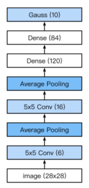
Access to data and training models
Let's implement the LeNet model. We still use fashion MNIST as the training data set.
# data
batch_size = 256
train_iter, test_iter = d2l.load_data_fashion_mnist(
    batch_size=batch_size, root='/home/kesci/input/FashionMNIST2065')
print(len(train_iter))#235
In order to make the readers see the data more vividly, additional parts are added to show the image of the data
#Data display
import matplotlib.pyplot as plt
def show_fashion_mnist(images, labels):
    d2l.use_svg_display()
    # Here "UU" means we ignore (do not use) variables
    _, figs = plt.subplots(1, len(images), figsize=(12, 12))
    for f, img, lbl in zip(figs, images, labels):
        f.imshow(img.view((28, 28)).numpy())
        f.set_title(lbl)
        f.axes.get_xaxis().set_visible(False)
        f.axes.get_yaxis().set_visible(False)
    plt.show()

for Xdata,ylabel in train_iter:
    break
X, y = [], []
for i in range(10):
    print(Xdata[i].shape,ylabel[i].numpy())
    X.append(Xdata[i]) # Add the i th feature to X
    y.append(ylabel[i].numpy()) # Add the i-th label to y
show_fashion_mnist(X, y)
torch.Size([1, 28, 28]) 3
torch.Size([1, 28, 28]) 8
torch.Size([1, 28, 28]) 1
torch.Size([1, 28, 28]) 4
torch.Size([1, 28, 28]) 0
torch.Size([1, 28, 28]) 0
torch.Size([1, 28, 28]) 4
torch.Size([1, 28, 28]) 9
torch.Size([1, 28, 28]) 4
torch.Size([1, 28, 28]) 7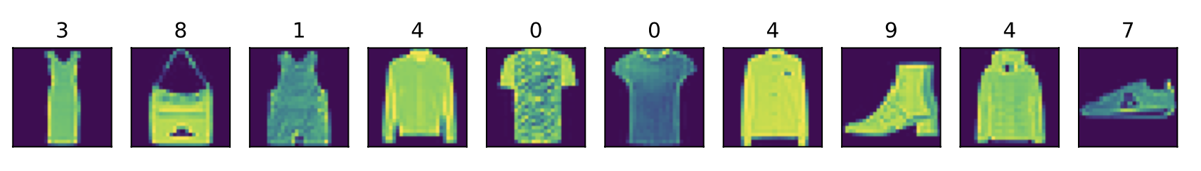
Because the computation of convolutional neural network is more complex than that of multi-layer perceptron, GPU is recommended to accelerate the computation. Let's check whether GPU can be used. If it succeeds, cuda:0 will be used, otherwise cpu will still be used.
# This function has been saved in the d2l package for future use
#use GPU
def try_gpu():
    """If GPU is available, return torch.device as cuda:0; else return torch.device as cpu."""
    if torch.cuda.is_available():
        device = torch.device('cuda:0')
    else:
        device = torch.device('cpu')
    return device

device = try_gpu()
device
device(type='cpu')
We implement the evaluate ﹣ accuracy function, which is used to calculate the accuracy of the model net on the dataset data ﹣ ITER.
#Calculation accuracy
'''
(1). net.train()
  //Enable BatchNormalization and Dropout and set BatchNormalization and Dropout to True
(2). net.eval()
//Do not enable BatchNormalization and Dropout, set BatchNormalization and Dropout to False
'''

def evaluate_accuracy(data_iter, net,device=torch.device('cpu')):
    """Evaluate accuracy of a model on the given data set."""
    acc_sum,n = torch.tensor([0],dtype=torch.float32,device=device),0
    for X,y in data_iter:
        # If device is the GPU, copy the data to the GPU.
        X,y = X.to(device),y.to(device)
        net.eval()
        with torch.no_grad():
            y = y.long()
            acc_sum += torch.sum((torch.argmax(net(X), dim=1) == y))  #[[0.2 ,0.4 ,0.5 ,0.6 ,0.8] ,[ 0.1,0.2 ,0.4 ,0.3 ,0.1]] => [ 4 , 2 ]
            n += y.shape[0]
    return acc_sum.item()/n
We define the function train to train the model.
#Training function
def train_ch5(net, train_iter, test_iter,criterion, num_epochs, batch_size, device,lr=None):
    """Train and evaluate a model with CPU or GPU."""
    print('training on', device)
    net.to(device)
    optimizer = optim.SGD(net.parameters(), lr=lr)
    for epoch in range(num_epochs):
        train_l_sum = torch.tensor([0.0],dtype=torch.float32,device=device)
        train_acc_sum = torch.tensor([0.0],dtype=torch.float32,device=device)
        n, start = 0, time.time()
        for X, y in train_iter:
            net.train()

            optimizer.zero_grad()
            X,y = X.to(device),y.to(device)
            y_hat = net(X)
            loss = criterion(y_hat, y)
            loss.backward()
            optimizer.step()

            with torch.no_grad():
                y = y.long()
                train_l_sum += loss.float()
                train_acc_sum += (torch.sum((torch.argmax(y_hat, dim=1) == y))).float()
                n += y.shape[0]
        test_acc = evaluate_accuracy(test_iter, net,device)
        print('epoch %d, loss %.4f, train acc %.3f, test acc %.3f, '
              'time %.1f sec'
              % (epoch + 1, train_l_sum/n, train_acc_sum/n, test_acc,
                 time.time() - start))
We reinitialize the model parameters to the corresponding device(cpu or cuda:0), and use Xavier for random initialization. Loss function and training algorithm still use cross entropy loss function and small batch random gradient descent.
# train
lr, num_epochs = 0.9, 10

def init_weights(m):
    if type(m) == nn.Linear or type(m) == nn.Conv2d:
        torch.nn.init.xavier_uniform_(m.weight)

net.apply(init_weights)
net = net.to(device)

criterion = nn.CrossEntropyLoss()   #Cross entropy describes the distance between two probability distributions. The more cross entropy is, the closer they are
train_ch5(net, train_iter, test_iter, criterion,num_epochs, batch_size,device, lr)
training on cpu
epoch 1, loss 0.0091, train acc 0.100, test acc 0.168, time 21.6 sec
epoch 2, loss 0.0065, train acc 0.355, test acc 0.599, time 21.5 sec
epoch 3, loss 0.0035, train acc 0.651, test acc 0.665, time 21.8 sec
epoch 4, loss 0.0028, train acc 0.717, test acc 0.723, time 21.7 sec
epoch 5, loss 0.0025, train acc 0.746, test acc 0.753, time 21.4 sec
epoch 6, loss 0.0023, train acc 0.767, test acc 0.754, time 21.5 sec
epoch 7, loss 0.0022, train acc 0.782, test acc 0.785, time 21.3 sec
epoch 8, loss 0.0021, train acc 0.798, test acc 0.791, time 21.8 sec
epoch 9, loss 0.0019, train acc 0.811, test acc 0.790, time 22.0 sec
epoch 10, loss 0.0019, train acc 0.821, test acc 0.804, time 22.1 sec
# test
for testdata,testlabe in test_iter:
    testdata,testlabe = testdata.to(device),testlabe.to(device)
    break
print(testdata.shape,testlabe.shape)
net.eval()
y_pre = net(testdata)
print(torch.argmax(y_pre,dim=1)[:10])
print(testlabe[:10])
torch.Size([256, 1, 28, 28]) torch.Size([256])
tensor([9, 2, 1, 1, 6, 1, 2, 6, 5, 7])
tensor([9, 2, 1, 1, 6, 1, 4, 6, 5, 7])
Conclusion:
Convolution neural network is a network with convolution layer. LeNet alternately uses convolution layer and maximum pooling layer followed by full connection layer for image classification.

