day4 - classification problems (understanding and sharing of relevant case codes)

experience

On the fourth day of team study, datawhale, an open source learning organization, used sklearn to build a complete classification project, reviewed some classification models in machine learning, practiced the calling codes of relevant models, annotated and understood all the codes, and completed the arranged homework tasks. Here, I thank the partners of datawhale open source community for their learning help, The future study should be the same. Come on

Tip: the following is the main content of this article. The following cases and knowledge points are provided by datawhale open source organization

preface

1, Use sklearn to build a complete classification project

1. Collect data sets and select appropriate features

from sklearn import datasets
iris = datasets.load_iris()
X = iris.data
y = iris.target
feature = iris.feature_names
data = pd.DataFrame(X,columns=feature)
data['target'] = y
data.head()

2. Select metrics to measure model performance

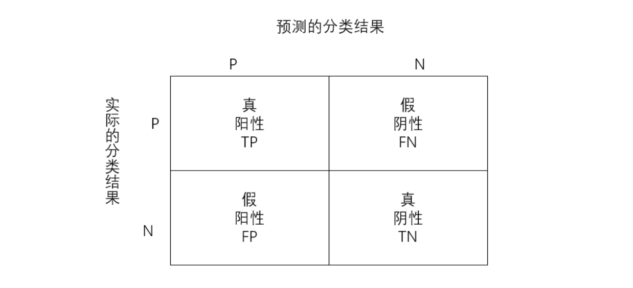
• True positive TP: both predicted value and true value are positive examples;

• True negative TN: both predicted and true values were positive;

• False positive FP: the predicted value is positive and the actual value is negative;

• False negative FN: the predicted value is negative and the actual value is positive;
  

• Accuracy: the proportion of correctly classified samples in the total samples
  

• Accuracy: the proportion of samples with positive prediction and correct classification in the positive prediction value
  

• Recall rate: proportion of samples with positive prediction and correct classification in positive category
  

• F1 value: comprehensive measurement accuracy and recall rate
  

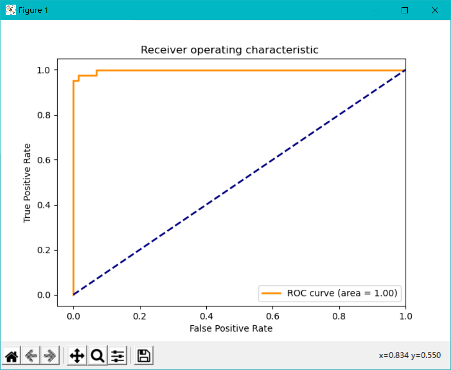
• ROC curve: the curve drawn with false positive rate as the horizontal axis and true positive rate as the vertical axis. The larger the area below the curve, the better.

3. Select specific models and train them

(1) logistic regression

We assume that the logistic regression model is:

Let's deduce the logistic regression model:

Because y can only take 0 or 1, it is assumed that the data obey 0-1 distribution, also known as Bernoulli distribution,

As like as two peas, you can bring in y=0 and y=1 to verify it, and the result is exactly the same as the previous conclusion.
We use maximum likelihood to estimate MLE, that is:

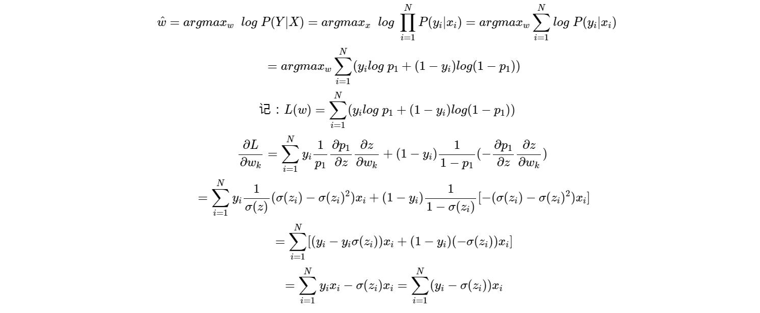
therefore

Since the functions involved here can not simply obtain the analytical solution like linear regression, we use the iterative optimization algorithm: gradient descent method, that is:

It is worth noting that logistic regression is not used for multi classification problems in practice, because the actual effect is not very good

(2) Probability based classification model

(a) Linear discriminant analysis

When classifying based on data, a natural idea is to reduce the dimension of high-dimensional data to one dimension, and then use a certain threshold to separate each category. The following is shown in the form of figure:

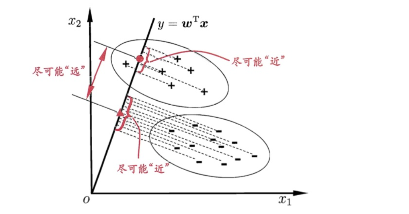
In the figure, the dimension of the data is two-dimensional. Our idea is to reduce the dimension of the data to one-dimensional, and then classify it with a threshold. This seems to be a good idea. We always hope that the internal variance of the same category of data after dimensionality reduction is small, and the variance between different categories should be as large as possible. This is also reasonable, because the data of the same category should be more similar, so the variance is small; Different types of data should be very different, so that it is easier to classify the data. We call it short: small intra class variance and large inter class variance. It is called "loose coupling and high cohesion" in computer language. Before specific derivation, we will describe the form of data and some basic statistics:

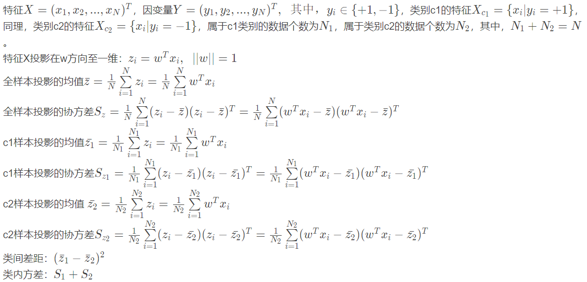
Since the objective of linear discriminant analysis is that the variance within the same category is small and the distance between different categories is large, the loss function is defined as:

(b) Naive Bayes

In linear discriminant analysis, we assume that the features under each classification category follow the same covariance matrix, and there is covariance between each two features. Therefore, in linear discriminant analysis, whether various features are independent or not. However, naive Bayes algorithm further simplifies the model of linear discriminant analysis. It turns all the covariances in the covariance matrix in linear discriminant analysis into 0, and only retains the variance of their respective features, that is, naive Bayes assumes that there is no correlation between each feature. In the deviation variance theory seen before, we know that the simplification of the model can reduce the variance, but increase the deviation. Therefore, naive Bayes is no exception. It has smaller variance and larger deviation than the linear discriminant analysis model. Although the model is simplified, there are many cases using naive Bayes in practice, even more than linear discriminant analysis, such as famous news classification, spam classification and so on.

(3) Decision tree

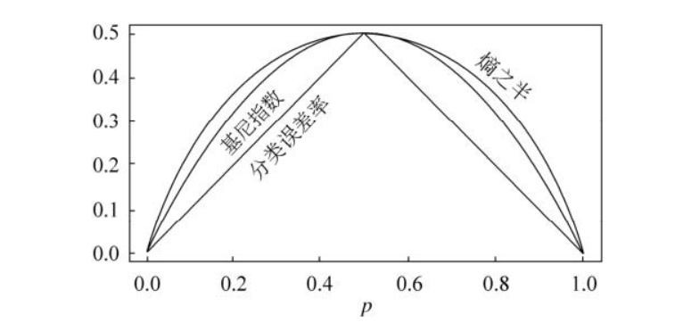
In the regression tree, for a given observation value, the predicted value of the dependent variable takes the average dependent variable of the training set in the terminal node to which it belongs. Correspondingly, for the classification tree, given an observation value, the predicted value of the dependent variable is the most common class of the training set in the terminal node to which it belongs. The construction process of classification tree is also very similar to that of regression tree. Like regression tree, classification tree also adopts recursive binary splitting. However, in the classification tree, the mean square error can not be used as the criterion to determine the split node. A natural alternative index is the classification error rate. Classification error rate refers to the category occupied by non common classes in the training set in this area, namely:

p ^ m k in the above formula represents the proportion of class k in the training set of region M. However, a large number of facts have proved that the classification error rate is not sensitive enough when building the decision tree. In practice, it is generally replaced by the following two indicators:
(1) Gini coefficient:

In the definition of Gini coefficient, we find that this index measures the total variance of K categories. It is not difficult to find that if all the values of p ^ m k are close to 0 or 1, the Gini coefficient will be very small. Therefore, Gini coefficient is regarded as an index to measure the purity of nodes - if its value is small, it means that a node contains observations from almost the same category.
The classification tree obtained by using Gini coefficient as an index is called CART.
(2) Cross entropy:
The index that can replace Gini coefficient is cross entropy, which is defined as follows:

Obviously, if all p ^ m k are close to 0 or 1, the cross entropy will be close to 0. Therefore, like the Gini coefficient, the higher the purity of the m-th node, the smaller the cross entropy. It is proved that Gini coefficient and cross entropy are very close in value.

Complete steps of decision tree classification algorithm:
a. Select the optimal segmentation feature j and the best advantage s on the feature:
After traversing the feature j and fixed j, traversing the segmentation point s, select the (j,s) that minimizes the Gini coefficient or cross entropy
b. According to (j,s) splitting feature space, the category in each region is the category with the largest proportion of samples in the region.
c. Continue to call steps 1 and 2 until the stop condition is met, that is, the number of samples in each region is less than or equal to 5.
d. The feature space is divided into J different regions to generate a classification tree.

(4) Support vector machine SVM

Support vector machine SVM is a classification algorithm developed in the computer industry in the 1990s. It has been proved to have good results in many problems. It is considered to be one of the most adaptive algorithms.

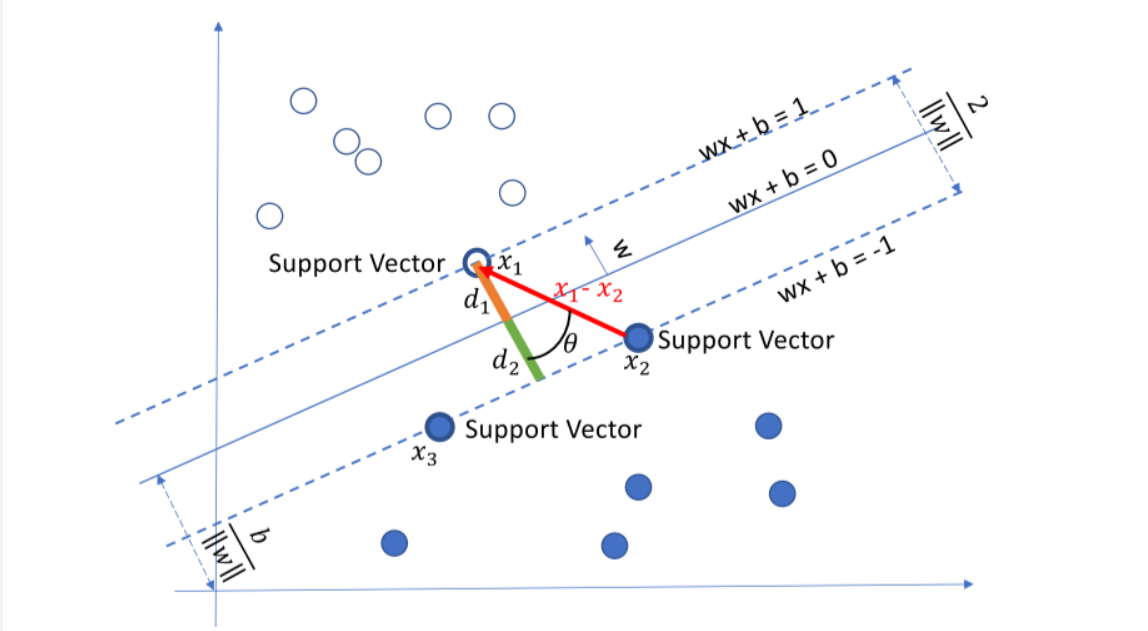
The basic principle of support vector machine is very simple. As shown in the figure, white and blue points belong to one category respectively. Our goal is to find a segmentation plane to separate the two categories. Generally speaking, if the data itself is linearly separable, there are actually countless such hyperplanes. This is because given a split plane, moving up and down or rotating the hyperplane slightly, the data can still be separated as long as it does not contact these observation points. A very natural idea is to find the maximum spacing hyperplane, that is, to find a partition plane farthest from the nearest observation point.

Specific form of SVM model:

The above discusses how linear support vector machine works, but in real life, it is difficult to encounter linearly separable data sets If we use the above formula to expand low-dimensional data to high-dimensional data, we must face a big problem, that is, the amount of calculation caused by dimension explosion is too large. Can we avoid this problem? Kernel functions are on the stage. Here are several common kernel functions:
(1) Polynomial kernel function:

C is used to control the strength of the lower order term. C = 0 and d = 1 represent the non kernel function.
(2) Gaussian kernel function:
Gaussian Kernel, also known as radial basis function (RBF) in SVM, is the most mainstream kernel function of nonlinear classification SVM. It is the default kernel function of libsvm. The expression is:
Before using Gaussian kernel function, we need to standardize the features, so here we measure the similarity between samples.
(3) Sigmoid kernel function:
The Sigmoid Kernel is also one of the commonly used kernel functions of linear non separable SVM. The expression is:

At this time, SVM is equivalent to a simple neural network without hidden layer.
(4) Cosine similarity kernel:
It is commonly used to measure the cosine similarity of two paragraphs of text. The expression is:

2, Example

1. Logistic regression:

'''
penalty {'l1', 'l2', 'elasticnet', 'none'}, default='l2'Regularization method
dual     bool type, default=False   Whether to use dual form, when n_samples> n_features Default when dual = False. 
C        float type, default=1.0
solver   {'newton-cg', 'lbfgs', 'liblinear', 'sag', 'saga'}, default='lbfgs'
l1_ratio float type, default=None
'''
from sklearn.linear_model import LogisticRegression
log_iris = LogisticRegression()
log_iris.fit(X,y)
log_iris.score(X,y)

2. Linear discriminant analysis:

'''
Parameters:
solver:{'svd'，'lsqr'，'eigen'}，default='svd'
solver Use of, possible values:
'svd': Singular value decomposition (default). The covariance matrix is not calculated, so it is recommended to use this solver for data with large characteristics.
'lsqr': The least squares solution can be used in combination with shrinkage.
'eigen': Eigenvalue decomposition can be used in combination with shrinkage.
'''
from sklearn.discriminant_analysis import LinearDiscriminantAnalysis
lda_iris = LinearDiscriminantAnalysis()
lda_iris.fit(X,y)
lda_iris.score(X,y)

3. Naive Bayes:

from sklearn.naive_bayes import GaussianNB
NB_iris = GaussianNB()
NB_iris.fit(X, y)
NB_iris.score(X,y)

4. iris is classified by decision tree algorithm:

'''
criterion:{"gini", "entropy"}, default="gini"
max_depth:The maximum depth of the tree.
min_samples_split:Minimum number of samples required to split internal nodes
min_samples_leaf :The minimum number of samples required at the leaf node.
'''
from sklearn.tree import DecisionTreeClassifier
tree_iris = DecisionTreeClassifier(min_samples_leaf=5)
tree_iris.fit(X,y)
tree_iris.score(X,y)

5. Support vector machine SVM:

from sklearn.pipeline import make_pipeline
from sklearn.preprocessing import StandardScaler
from sklearn.svm import SVC
'''
C:Regularization parameters. Strength and of regularization C Inversely proportional. Must be strictly positive. The penalty is square l2 Punishment.
kernel:{'linear'，'poly'，'rbf'，'sigmoid'，'precomputed'}，default='rbf'
degree:Order of polynomial sum
gamma:" rbf"，" poly"And“ Sigmoid"Kernel coefficient of.
shrinking:Soft interval classification, default true
'''
svc_iris = make_pipeline(StandardScaler(), SVC(gamma='auto'))
svc_iris.fit(X, y)
svc_iris.score(X,y)

6. Evaluate the performance of the model and adjust the parameters:

Method 1: grid searchgridsearchcv ()

from sklearn.model_selection import GridSearchCV
from sklearn.svm import SVC
import time

start_time = time.time()
pipe_svc = make_pipeline(StandardScaler(),SVC(random_state=1))
param_range = [0.0001,0.001,0.01,0.1,1.0,10.0,100.0,1000.0]
param_grid = [{'svc__C':param_range,'svc__kernel':['linear']},
              {'svc__C':param_range,'svc__gamma':param_range,'svc__kernel':['rbf']}]
'''
estimator: scikit-learn Classifier interface. Need scoring mechanism score()perhaps scoring Parameter setting
param_grid: The dictionary with parameter name (string) as key and the parameter setting list (or the list of such dictionaries) as value can search any parameter setting sequence;
scoring: String, default: none;
cv: Cross validation parameters(Several fold cross validation)
n_jobs: Parallel number, and CPU Kernel consistency
'''
gs = GridSearchCV(estimator=pipe_svc,param_grid=param_grid,scoring='accuracy',cv=10,n_jobs=-1)
gs = gs.fit(X,y)
end_time = time.time()

print("Grid search elapsed time:%.3f S" % float(end_time-start_time))
print(gs.best_score_)
print(gs.best_params_)

Method 2: random mesh search (randomizedsearchcv)

from sklearn.model_selection import RandomizedSearchCV
from sklearn.svm import SVC
import time

start_time = time.time()
pipe_svc = make_pipeline(StandardScaler(),SVC(random_state=1))
param_range = [0.0001,0.001,0.01,0.1,1.0,10.0,100.0,1000.0]
param_grid = [{'svc__C':param_range,'svc__kernel':['linear']},
              {'svc__C':param_range,'svc__gamma':param_range,'svc__kernel':['rbf']}]
# param_grid = [{'svc__C':param_range,'svc__kernel':['linear','rbf'],'svc__gamma':param_range}]

gs = RandomizedSearchCV(estimator=pipe_svc, param_distributions=param_grid,scoring='accuracy',cv=10,n_jobs=-1)
gs = gs.fit(X,y)
end_time = time.time()

print("Random grid search elapsed time:%.3f S" % float(end_time-start_time))
print(gs.best_score_)
print(gs.best_params_)

7. When the categories are two, the confusion matrix and ROC curve can be drawn:

Confusion matrix:

# Load data
df = pd.read_csv("http://archive.ics.uci.edu/ml/machine-learning-databases/breast-cancer-wisconsin/wdbc.data",header=None)
'''
Breast cancer dataset: 569 samples of malignant and benign tumor cells. M Is malignant, B Benign
'''

import matplotlib
# The backend of matplotlib uses the default configuration of agg. Pictures cannot be displayed at this time. Change the setting to TkAgg
matplotlib.use('TkAgg')
from matplotlib import pyplot as plt

# Do basic data preprocessing
from sklearn.preprocessing import LabelEncoder

X = df.iloc[:,2:].values
y = df.iloc[:,1].values
le = LabelEncoder()    #Encode M-B and other strings into 0-1 that can be recognized by the computer
y = le.fit_transform(y)
le.transform(['M','B'])

# Data segmentation 8:2
from sklearn.model_selection import train_test_split

X_train,X_test,y_train,y_test = train_test_split(X,y,test_size=0.2,stratify=y,random_state=1)
from sklearn.svm import SVC
pipe_svc = make_pipeline(StandardScaler(),SVC(random_state=1))
from sklearn.metrics import confusion_matrix

pipe_svc.fit(X_train,y_train)
y_pred = pipe_svc.predict(X_test)
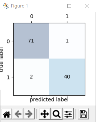
# The confusion matrix was calculated to evaluate the accuracy of classification.
confmat = confusion_matrix(y_true=y_test,y_pred=y_pred)

'''
subplots Parameter introduction:
figsize=(2.5,2.5) ，The image size is set.
Return value:
fig: matplotlib.figure.Figure object
 ax: Subgraph object( matplotlib.axes.Axes)Or his array
'''
fig,ax = plt.subplots(figsize=(2.5,2.5))


'''
matshow(A,cmap,alpha)Parameter introduction:
A Is the matrix, and the confusion matrix just calculated is passed in here
cmap Set color
'''
ax.matshow(confmat, cmap=plt.cm.Blues,alpha=0.3)
for i in range(confmat.shape[0]):
    for j in range(confmat.shape[1]):
        ax.text(x=j,y=i,s=confmat[i,j],va='center',ha='center')
plt.xlabel('predicted label')
plt.ylabel('true label')
plt.show()

Draw ROC curve:

from sklearn.metrics import roc_curve,auc
from sklearn.metrics import make_scorer,f1_score

# Score here with f1
scorer = make_scorer(f1_score,pos_label=0)
# Perform grid search
gs = GridSearchCV(estimator=pipe_svc,param_grid=param_grid,scoring=scorer,cv=10)

'''
decision_function
 Indicates that the confidence is expressed by measuring the distance between the sample distance and the separation hyperplane
 Calculate the decision value of the classifier on the test set
 Usage can refer to the article: https://blog.csdn.net/cxx654/article/details/106727812
'''
y_pred = gs.fit(X_train,y_train).decision_function(X_test)
#y_pred = gs.predict(X_test)

# Calculate the true positive rate and false positive rate
fpr,tpr,threshold = roc_curve(y_test, y_pred)
# Calculate the value of auc
roc_auc = auc(fpr,tpr)

lw = 2
plt.figure(figsize=(7,5))
plt.plot(fpr, tpr, color='darkorange',
         lw=lw, label='ROC curve (area = %0.2f)' % roc_auc) ###The false positive rate is the abscissa and the true positive rate is the ordinate
plt.plot([0, 1], [0, 1], color='navy', lw=lw, linestyle='--')
plt.xlim([-0.05, 1.0])
plt.ylim([-0.05, 1.05])
plt.xlabel('False Positive Rate')
plt.ylabel('True Positive Rate')
plt.title('Receiver operating characteristic ')
plt.legend(loc="lower right")
plt.show()

3, Homework

(1) The relationship and difference between regression problem and classification problem, and how to use regression problem to understand classification problem

difference:

• Classification is the task of predicting a discrete label. Classification prediction can be evaluated by accuracy, while regression problem can not
• Regression is to predict a continuous number of tasks. Regression prediction can be evaluated by root mean square error, but classification can not.

Contact:

• The classification algorithm may predict a continuous value, but these continuous values correspond to the form of probability of a category.
• The regression algorithm can predict the discrete value, but it can predict the discrete value in the form of integer quantity.

Using regression problem to understand classification problem

In some cases, regression problems can be transformed into classification problems. For example, the predicted quantity is a range that can be converted into discrete values. Amounts between $0 and $100 can be divided into two ranges:
class 0: $0 to $49
class 1: to $100
This is usually called discretization. The output variables in the result are a classification, and the labels of the classification are sequential (called ordinal numbers).

We transform the continuous numerical value into a range interval, that is, the discrete numerical interval, and transform the regression problem into a classification problem.

reference resources: https://www.jiqizhixin.com/articles/2017-12-15-2

(2) Why can the loss function of classification problem be cross entropy rather than mean square error

Cross entropy Loss and mean square deviation Loss are defined as follows:

The derivative of w in the two loss functions is obtained by gradient descent method:

It can be seen that the derivative sigmoid is very small when the output is close to 0 and 1, so the model parameter w will learn very slowly when using the minimum mean square deviation Loss. Using cross entropy Loss does not have this problem. For faster learning speed, the cross entropy Loss function is generally used in classification problems.

reference resources: https://zhuanlan.zhihu.com/p/104130889

(3) What are the similarities and differences between linear discriminant analysis and logistic regression in estimating parameters

• Difference: LDA needs to assume normal distribution, calculate the mean and covariance matrix according to the sample, and then bring it into the discriminant. LogitsR uses maximum log likelihood to estimate parameters.
• Same: all variables are input to each class

(4) Attempt to derive SVM from 0

In support vector machine, we use margin to describe the distance between the partition hyperplane and the sample. Before introducing spacing, we need to know how to calculate the distance from the midpoint of space to the plane. The distance from a point p ∈ r in R d space to hyperplane w ⊤ x + b = 0 is:

The interval represents twice the distance from the sample closest to the partition hyperplane to the partition hyperplane, i.e

The goal of linear support vector machine is to find a suitable set of parameters (w; b) so that

But this problem is very complex and difficult to deal with In order to be applied in reality, we hope to simplify it. Since the scaling of (w; b) does not affect the solution, in order to simplify the optimization problem, we constrain (w; b) so that:

Therefore, the problem of our linear support vector machine can be restated as: finding a set of appropriate parameters (w; b), so that

The form written as Lagrange function is:

The dual problem of linear support vector machine is equivalent to finding a set of appropriate parameters α, So that the dual problem is:

By derivation:

The final optimization problem can be obtained by substituting the derivative result into the dual problem:

(5) The relationship and difference between quadratic discriminant analysis, linear discriminant analysis and naive Bayes

• Linear discriminant analysis (LDA) constructs a linear decision plane and quadratic discriminant analysis (QDA) constructs a quadratic decision plane. These classifiers can easily calculate the analytical solution (referring to the solution obtained through strict formula), which has the characteristics of multi classification and does not need parameters in practice. The difference between linear discriminant analysis and quadratic discriminant analysis is that quadratic discriminant analysis can learn quadratic boundary and the model is more flexible.

• Naive Bayes is a generative model. Naive Bayes classifier is based on Bayes theorem and assumes that all features are independent of each other. LDA and QDA do not require it.

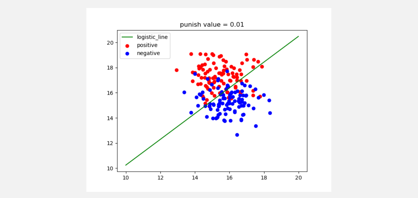
(6) Using python+numpy to realize logical regression

#!/usr/bin/env python3
# -*- coding: utf-8 -*-
# @Time: 21 / 8 / 22 12:34 by Zhou Jianguo

from math import exp
import matplotlib.pyplot as plt
import numpy as np
from sklearn.datasets.samples_generator import make_blobs


def sigmoid(num):
    '''

    :param num: To be calculated x
    :return: sigmoid Subsequent values
    '''
    if type(num) == int or type(num) == float:
        return 1.0 / (1 + exp(-1 * num))
#   else:
#       raise ValueError, 'only int or float data can compute sigmoid'


class logistic():
    def __init__(self, x, y):
        if type(x) == type(y) == list:
            self.x = np.array(x)
            self.y = np.array(y)
        elif type(x) == type(y) == np.ndarray:
            self.x = x
            self.y = y
#         else:
#             raise ValueError, 'input data error'

    def sigmoid(self,x):
        '''
        :param x: Input vector
        :return: The input vector as a whole simgoid Calculated vector result
        '''
        s = np.frompyfunc(lambda x: sigmoid(x), 1, 1)
        #The second parameter is the number of parameters in func, and the third parameter is the number of return values in func
        return s(x)

    def train_with_punish(self, alpha, errors, punish=0.0001):
        '''
        :param alpha: alpha Is the learning rate
        :param errors: The threshold to stop the iteration when the error is less than what
        :param punish: Penalty coefficient
        :param times: Maximum number of iterations
        :return:
        '''
        self.punish = punish
        dimension = self.x.shape[1]
        self.theta = np.random.random(dimension)
        compute_error = 100000000
        times = 0
        while compute_error > errors:
            res = np.dot(self.x, self.theta)
            delta = self.sigmoid(res) - self.y
            self.theta = self.theta - alpha * np.dot(self.x.T, delta) - punish * self.theta  # Gradient descent method with penalty
            compute_error = np.sum(delta)
            times += 1

    def predict(self, x):
        '''
        :param x: Give in a new unlabeled vector
        :return: Return the determined category according to the calculated parameters
        '''
        x = np.array(x)
        if self.sigmoid(np.dot(x, self.theta)) > 0.5:
            return 1
        else:
            return 0


def test1():
    '''
    Used for testing and drawing to show the effect
    :return:
    '''
    x, y = make_blobs(n_samples=200, centers=2, n_features=2, random_state=0, center_box=(10, 20))
    x1 = []
    y1 = []
    x2 = []
    y2 = []
    for i in range(len(y)):
        if y[i] == 0:
            x1.append(x[i][0])
            y1.append(x[i][1])
        elif y[i] == 1:
            x2.append(x[i][0])
            y2.append(x[i][1])
    # The above data are processed and two types of data are generated
    p = logistic(x, y)
    p.train_with_punish(alpha=0.00001, errors=0.005, punish=0.01)  # The step size is 0.00001, the maximum allowable error is 0.005, and the penalty coefficient is 0.01
    x_test = np.arange(10, 20, 0.01)
    y_test = (-1 * p.theta[0] / p.theta[1]) * x_test
    plt.plot(x_test, y_test, c='g', label='logistic_line')
    plt.scatter(x1, y1, c='r', label='positive')
    plt.scatter(x2, y2, c='b', label='negative')
    plt.legend(loc=2)
    plt.title('punish value = ' + p.punish.__str__())
    plt.show()


if __name__ == '__main__':
    test1()

(7) Understand the optimization algorithms such as gradient descent method, Newton method, quasi Newton method and SOM algorithm

• Gradient descent method: its essence is to select the descent direction d k only by using the first derivative information of the function. The most basic algorithm is the gradient descent method, that is, directly select the negative gradient as the descent direction D K
• Newton method: Newton algorithm is an algorithm that uses the second derivative information to construct the iterative format. Due to the use of more information, the actual performance of Newton method can be much better than gradient method, but its requirements for function f (x) also become higher
• Quasi Newton method: it can generate approximate matrix at less computational cost at each step, and the iterative sequence generated by using approximate matrix instead of heather matrix still has the property of superlinear convergence.
• SMO algorithm: sequence minimization (SMO) is an efficient optimization algorithm using the characteristics of support vector machine The basic idea of SMO is coordinate descent.

summary

The above is what I want to talk about today. This paper uses sklearn to build a complete classification project, reviews some classification models in machine learning, practices the calling code of relevant models, reproduces some cases, and makes my own understanding and comments. Here again, I thank the partners of datawhale open source community for their learning help, For more learning materials, please contact datawhale to participate in team learning.

Relevant data:
[1] Instructional Video: https://www.bilibili.com/video/BV1Mb4y1o7ck?from=search&seid=6085778383215596866
[2] Lesson plan: https://github.com/datawhalechina/ensemble-learning
[3] Datawhale open source learning community: http://datawhale.club/