4, HQL (hive SQL)
https://www.docs4dev.com/docs/zh/apache-hive/3.1.1/reference/#
1) Add the following configuration information to the hive-site.xml file to display the header information of the current database and query table.
<property>
	<name>hive.cli.print.header</name>
	<value>true</value>
</property>
<property>
	<name>hive.cli.print.current.db</name>
	<value>true</value>
</property>
2) Restart hive and compare the differences before and after configuration.
(1) Before configuration, as shown in the figure:
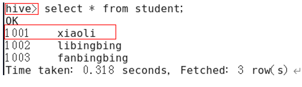
Figure 12-1 before configuration
(2) After configuration, as shown in the figure:
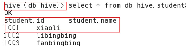
Figure 12-2 after configuration
(2) DML data manipulation language
1. Data import
(1) Directly upload data
--cursor
 No table file directory, unable to upload

--Internal table
hadoop fs -put emp.txt /user/hive/warehouse/offcn.db/managed_emp01/aaa.txt
hadoop fs -put student.txt /user/hive/warehouse/
select * from managed_emp01;

--External table
hadoop fs -put emp.txt /user/hive/warehouse/offcn.db/managed_emp/bbb.txt
select * from external_emp01;

--Partition table
hadoop fs -put emp.txt /user/hive/warehouse/offcn.db/partition_emp/age=20/
select * from partition_emp;
hadoop fs -put emp.txt /user/hive/warehouse/offcn.db/partition_emp2/month=5/day=20
select * from partition_emp2;
Note: after creating the partition table, manually create the partition field directory( mkdir),After uploading the data again, you need to repair the table before you can use it msck repair table tabName;

--Barrel table
hadoop fs -put emp.txt /user/hive/warehouse/offcn.db/buck_emp
select * from buck_emp;
We found that HDFS The file directory on is not divided into multiple files, that is, it is not divided into buckets according to the specified fields
(1) Load data into a table (load)
Syntax:
load data [local] inpath 'path/target.log' [overwrite] into table tab [partition (partcol1=val1,...)];
explain:
- load data: indicates loading data
- local: means to load (copy) data locally from (the node started by the server) to the hive table; otherwise, load (move) data from HDFS to the hive table
- inpath: indicates the path to load data
- Overwrite: it means to overwrite the existing data in the table; otherwise, it means to append
- into table: indicates which table to load
- tab: indicates the specific table name
- Partition: indicates to upload to the specified partition
Example:
--Load data for temporary tables
use offcn;
create temporary table if not exists temporary_emp(
id int, name string
)row format delimited fields terminated by '\t';

load data local inpath "/home/offcn/apps/hive-3.1.2/emp.txt" into table temporary_emp;
select * from temporary_emp;

--Load data locally for internal tables
load data local inpath "/home/offcn/apps/hive-3.1.2/emp.txt" into table managed_emp01;
load data local inpath "/home/offcn/apps/hive-3.1.2/emp.txt" overwrite into table managed_emp01;
select * from managed_emp01;
--For internal tables from hdfs Load data
 Upload the data to hdfs
[offcn@bd-offcn-01 hive-3.1.2]$ hadoop fs -put emp.txt /user/offcn
load data inpath "/user/offcn/emp.txt" overwrite into table managed_emp01;
select * from managed_emp01;


--Load data for external tables
load data local inpath "/home/offcn/apps/hive-3.1.2/emp.txt" into table external_emp01;
select * from external_emp01;

--Load data for partitioned tables (single partition)
load data local inpath "/home/offcn/apps/hive-3.1.2/emp.txt" into table partition_emp partition(age=18);
select * from partition_emp;

--Load data for partitioned tables (multi-level partitioning)
load data local inpath "/home/offcn/apps/hive-3.1.2/emp.txt" into table partition_emp2 partition(month="05",day="20");
select * from partition_emp2;

--Load data for bucket table
load data local inpath "/home/offcn/apps/hive-3.1.2/emp.txt" into table buck_emp; Error loading method, unable to query data
select * from buck_emp;
[offcn@bd-offcn-01 hive-3.1.2]$ hadoop fs -put emp.txt /user/offcn
load data inpath "/user/offcn/emp.txt" into table buck_emp; If the data is queried by the correct loading method, this method will be retained/user/offcn/emp.txt file
select * from buck_emp;
Conclusion:
1,	Barrel distribution table passed load Load data, only hdfs Data on cannot be loaded. There is no local data,
2,	stay hdfs web When viewing the file content on the page, it is found that there is a problem with the display, which is hadoop of bug,To view the bucket file, you can use hadoop -cat command
3,	In case of this error, barrel separation will not be affected
(2) Insert data into a table through a query statement (insert)
a.insert values
Syntax:
insert into table tab [partition (partcol1[=val1], partcol2[=val2] ...)] values (value [, value ...])
Example:
b.insert select
Syntax:
insert overwrite table tablename [partition (partcol1=val1, partcol2=val2 ...)] select_statement1 from from_statement;
insert into table tablename [partition (partcol1=val1, partcol2=val2 ...)] select_statement1 from from_statement;
Example:
--Prepare the data first
insert into table emp02(id,name) values(4,"scala");
select * from emp02;

--cursor
insert overwrite table temporary_emp select * from emp02;  Overlay insert
insert into table temporary_emp select * from emp02;   New insert
--Internal table
insert into table managed_emp01 select * from emp02;
select * from managed_emp01;

--External table
insert into table external_emp01 select * from emp02;
select * from external_emp01;

--Partition table
insert into table partition_emp partition(age=45) select * from emp02;
select * from partition_emp;
insert into table partition_emp2 partition(month="3",day="18") select * from emp02;[X Column mismatch]
insert into table partition_emp2 partition(month="3",day="18") select * from partition_emp;
select * from partition_emp2;

--Barrel table
insert into table buck_emp select * from partition_emp;
select * from  buck_emp;
c. Multiple insertion
Syntax:
from from_statement
insert overwrite table tab [partition (partcol1=val1, partcol2=val2 ...)] select_statement1
[insert overwrite table tab2 [partition ...] select_statement2]
[insert into table tab2 [partition ...] select_statement2];
explain:
- When we need to insert part of the data in one table into multiple tables, we can use multiple inserts.
Example:
take partition_emp Some data in the table are inserted and replaced into managed_emp01,external_emp01 In the table:
-- Look at the original data first
select * from managed_emp01;  corresponding/user/hive/warehouse/offcn.db/managed_emp01
select * from external_emp01;  corresponding/user/hive/warehouse/offcn.db/managed_emp
select * from partition_emp;   corresponding/user/hive/warehouse/offcn.db/partition_emp

-- Execute insert
from partition_emp
insert into table managed_emp01
select id,name
insert overwrite table external_emp01
select id,name;
d. Dynamic partition
Syntax:
insert overwrite table tablename partition (partcol1[=val1], partcol2[=val2] ...) select_statement from from_statement;
insert into table tablename partition (partcol1[=val1], partcol2[=val2] ...) select_statement from from_statement;
explain:
- When inserting data into the hive partition table, if you need to create many partitions, such as partition storage with a field in the table, you need to copy, paste and modify many sql to execute, which is inefficient. Because hive is a batch processing system, hive provides a dynamic partition function, which can infer the partition name based on the location of query parameters, so as to establish the partition.
Example:
--Set non strict mode
set hive.exec.dynamic.partition.mode=nonstrict;
--Create dynamic partition table
create table dynamic_emp(id int) partitioned
by (name string) row format delimited fields terminated by '\t';
--Insert data dynamically
insert overwrite table dynamic_emp partition(name)
select id,name from managed_emp01;
--View all partitions
show partitions dynamic_emp;
--View data
select * from dynamic_emp;
(3) When creating a table, specify the load data path through Location
create table if not exists emp4(
id int, name string
)
row format delimited fields terminated by '\t'
location '/test';
hadoop fs -put emp.txt /test
select * from emp4;
(4) Import data into the specified Hive table
create table if not exists emp5(
id int, name string
)
row format delimited fields terminated by '\t';

import table emp5 from '/tmp/export/emp/';
select * from emp5;
Note: export the data first, then import and export it export It can only be used together
2. Data export
(1) Insert export
a. Export query results to local
insert overwrite local directory '/home/offcn/tmp/export/emp'
select * from managed_emp01;
b. Format and export query results to local
insert overwrite local directory '/home/offcn/tmp/export/emp2'
ROW FORMAT DELIMITED FIELDS TERMINATED BY '\t'
select * from managed_emp01;
c. Export the query results to HDFS (no local)
insert overwrite directory '/test/export/empout'
ROW FORMAT DELIMITED FIELDS TERMINATED BY '\t'
select * from managed_emp01;
(2) Hadoop command export to local
 jdbc:hive2://bd-offcn-01:10000>  dfs -get /user/hive/warehouse/offcn.db/emp5/emp.txt /home/offcn/tmp/export/emp2/emp.txt;
Or use it directly hadoop Command to download the corresponding file locally
(3) Hive Shell command export
hive -e 'select * from offcn.emp02;' > /home/offcn/tmp/export/emp.txt
(4) Export to HDFS
export table offcn.emp02 to
'/tmp/export/emp';
export and import are mainly used for Hive table migration between two Hadoop platform clusters.
(3) DQL data query language
Data preparation:
use default;

create table if not exists emp(
empno int,
ename string,
job string,
mgr int,
hiredate string,
sal double,
comm double,
deptno int)
row format delimited fields terminated by '\t';


create table if not exists dept(
deptno int,
dname string,
loc int
)
row format delimited fields terminated by '\t';

load data local inpath '/home/offcn/tmp/emp.txt' into table emp;
load data local inpath '/home/offcn/tmp/dept.txt' into table dept;

select * from emp;
select * from dept;
1. Basic query (Select... From)
Full table query
select * from emp;
Select a specific column query
select empno, ename from emp;
be careful:
- SQL language is case insensitive.
- SQL can be written on one or more lines
- Keywords cannot be abbreviated or broken
- Each clause should be written separately.
- Use indentation to improve the readability of statements.
2. Condition query
Query all employees whose salary is greater than 1000
select * from emp where sal >1000;
Relational operator
| Operator | Supported data types | describe |
| A=B | Basic data type | If A is equal to B, it returns TRUE, otherwise it returns FALSE |
| A<=>B | Basic data type | Returns TRUE if both A and B are NULL, and False if one side is NULL |
| A<>B, A!=B | Basic data type | If A or B is NULL, NULL is returned; if A is not equal to B, TRUE is returned; otherwise, FALSE is returned |
| A<B | Basic data type | If A or B is NULL, NULL is returned; if A is less than B, TRUE is returned; otherwise, FALSE is returned |
| A<=B | Basic data type | If A or B is NULL, NULL is returned; if A is less than or equal to B, TRUE is returned; otherwise, FALSE is returned |
| A>B | Basic data type | If A or B is NULL, NULL is returned; if A is greater than B, TRUE is returned; otherwise, FALSE is returned |
| A>=B | Basic data type | If A or B is NULL, NULL is returned; if A is greater than or equal to B, TRUE is returned; otherwise, FALSE is returned |
| A [NOT] BETWEEN B AND C | Basic data type | If any of A, B or C is NULL, the result is NULL. If the value of A is greater than or equal to B and less than or equal to C, the result is TRUE, otherwise it is FALSE. If you use the NOT keyword, the opposite effect can be achieved. |
| A IS NULL | All data types | If A is equal to NULL, it returns TRUE, otherwise it returns FALSE |
| A IS NOT NULL | All data types | If A is not equal to NULL, it returns TRUE, otherwise it returns FALSE |
| In (value 1, value 2) | All data types | Use the IN operation to display the values IN the list |
| A [NOT] LIKE B | STRING type | B is A simple regular expression under SQL, also known as wildcard pattern. If A matches it, it returns TRUE; otherwise, it returns FALSE. The expression description of B is as follows: 'x%' means that A must start with the letter 'x', '% X' means that A must end with the letter 'x', and '% X%' means that A contains the letter 'x', which can be located at the beginning, end or in the middle of the string. For example If the NOT keyword is used, the opposite effect can be achieved. |
| A RLIKE B, A REGEXP B | STRING type | B is A java based regular expression. If A matches it, it returns TRUE; otherwise, it returns FALSE. The matching is implemented by the regular expression interface in JDK, because the regular expression is also based on its rules. For example, the regular expression must match the whole string A, not just its string. |
(1)Between,IN,is null
- Find out all employees whose salary is equal to 5000
select * from emp where sal =5000;
- Query employee information with salary between 500 and 1000
select * from emp where sal between 500 and 1000;
- Query all employee information with comm blank
select * from emp where comm is null;
- Query employee information with salary of 1500 or 5000
select * from emp where sal IN (1500, 5000);
(2) Like and RLike
The selection criteria can contain characters or numbers:
%Represents zero or more characters (any character).
_Represents a character.
RLIKE clause:
RLIKE clause is an extension of this function in Hive, which can specify matching conditions through the more powerful language of Java regular expression.
- Find employee information starting with "S"
select * from emp where ename LIKE 'S%';
- Find the employee information for the salary with the second value of "M"
select * from emp where ename LIKE '_M%';
- Find employee information with "I" in the name
select * from emp where ename RLIKE '[I]';
select * from emp where ename LIKE '%I%';
3) Logical operator (And/Or/Not)
Operator meaning
AND logical Union
OR Logical or
NOT logical no
- The inquiry salary is more than 1000, and the Department is 30
select * from emp where sal>1000 and deptno=30;
- The inquiry salary is greater than 1000, or the Department is 30
select * from emp where sal>1000 or deptno=30;
- Query employee information except 20 departments and 30 departments
select * from emp where deptno not IN(30, 20);
(4) limit statement
The limit clause is used to limit the number of rows returned. Unlike mysql, limit can only be followed by one parameter
select * from emp limit 5;
3. Grouping query
(1) Group By statement
The GROUP BY statement is usually used with an aggregate function to group one or more queued results, and then aggregate each group.
Note: in grouping statements, the fields after select can only be grouping fields or aggregate functions!
- Calculate the average salary of each department in emp table
select t.deptno, avg(t.sal) avg_sal from emp t group by t.deptno;
- Calculate emp the maximum salary for each position in each department
select t.deptno, t.job, max(t.sal) max_sal from emp t group by t.deptno, t.job;
(2) Having statement
Differences between having and where
Grouping functions cannot be written after where, but can be used after having.
where is used to filter data and having is used to filter results.
having is only used for group by group statistics statements.
- The average salary of each department is greater than 2000
Step 1: find the average salary of each department
select deptno, avg(sal) from emp group by deptno;
Part II: seek departments with an average salary of more than 2000 in each department
select deptno, avg(sal) avg_sal from emp group by deptno having avg_sal > 2000;
It can't be written like this
select deptno, avg(sal) avg_sal from emp group by deptno where avg_sal > 2000;
4. Connection query
Join occurs between multiple tables, including inner join (equivalent inner join and unequal inner join) and outer join (left outer join, right outer join, and all outer join)
Internal connection: only data meeting the conditions will be displayed.
External connection: all the data of a table will be displayed. If another table cannot match it, the related fields of the other table will be set to blank.
(1) Inner connection
select e.*,d.*
from emp e inner join dept d
on e.deptno=d.deptno;

intersect Intersection mode implementation
select e.*,d.*
from emp e left outer join dept d
on e.deptno=d.deptno
intersect
select e.*,d.*
from emp e right outer join dept d
on e.deptno=d.deptno;
(2) External connection
a. Left link
--Left connection
select e.*,d.*
from emp e left outer join dept d
on e.deptno=d.deptno;
b. Right connection
--Right connection
select e.*,d.*
from emp e right outer join dept d
on e.deptno=d.deptno;
c. Left unique
--The left table has, while the right table has no matching data
select e.*,d.*
from emp e left outer join dept d
on e.deptno=d.deptno
where d.deptno is null;
d. Right unique
--The right table has data, while the left table does not
select e.*,d.*
from emp e right outer join dept d
on e.deptno=d.deptno
where e.deptno is null;
e. Full connection
--Full connection
select e.*,d.*
from emp e full outer join dept d
on e.deptno=d.deptno;

--Full connection union
select e.*,d.*
from emp e left outer join dept d
on e.deptno=d.deptno
union
select e.*,d.*
from emp e right outer join dept d
on e.deptno=d.deptno;
f. Left and right unique
--Left and right unique
select e.*,d.*
from emp e full outer join dept d
on e.deptno=d.deptno
where e.deptno is null or d.deptno is null;

--Left and right unique union all
select e.*,d.dname,d.loc
from emp e left outer join dept d
on e.deptno=d.deptno
where d.deptno is null
union all
select e.empno ,e.ename ,e.job,e.mgr,e.hiredate,e.sal,e.comm,d.*
from emp e right outer join dept d
on e.deptno=d.deptno
where e.deptno is null;

--except/minus: Difference set implementation
select e.*,d.*
from emp e full outer join dept d
on e.deptno=d.deptno
except
select e.*,d.*
from emp e inner join dept d
on e.deptno=d.deptno;

select e.*,d.*
from emp e full outer join dept d
on e.deptno=d.deptno
minus
select e.*,d.*
from emp e inner join dept d
on e.deptno=d.deptno;
g. Cross connect
Cross connection: get Cartesian product, which can be written implicitly and explicitly
Plus the on condition, it is equivalent to inner connection
Implicit writing
select e.*,d.*
from emp e,dept d;
Explicit writing
select e.*,d.*
from emp e cross join dept d
on e.deptno=d.deptno;
h. Left semi join
When the records meet the judgment conditions in the on statement for the right table, only the records of the left table will be returned. When the left half is disconnected, the internal connection will be optimized. When a piece of data in the left table exists in the right table, hive will stop scanning. Therefore, the efficiency is higher than that of join, but only the fields of the left table can appear after the select and where keywords of the left half open connection, and the fields of the right table cannot appear. Hive does not support right half disconnect.
select *
from dept d left semi join emp e
on d.deptno=e.deptno;

select d.*
from dept d left semi join emp e
on d.deptno=e.deptno;

--It is similar to the result that the inner connection only returns the contents of the left table, but the efficiency is higher. It is equivalent to the result that the inner connection only returns the left table and de duplicates the left table, but the efficiency is higher than that of the inner connection
select d.*
from dept d inner join emp e
on d.deptno=e.deptno;
--Error example
select d.*,e.*
from dept d left semi join emp e
on d.deptno=e.deptno;
(3) Self connection
Prepare data:
CREATE TABLE `area` (
  `id` string NOT NULL,
  `area_code` string,
  `area_name` string,
  `level` string,
  `parent_code` string,
  `target` string
)row format delimited fields terminated by ',';

load data local inpath "/home/offcn/tmp/area.csv" into table area;

select * from area;

Demand: Statistics of all regions under designated provinces and cities
--Subquery implementation
SELECT * FROM AREA
WHERE parent_code=(SELECT area_code
FROM AREA
WHERE area_name="Inner Mongolia Autonomous Region");
--Self connection implementation
SELECT a.*,b.area_name
FROM AREA a JOIN AREA b
ON a.parent_code=b.area_code
WHERE b.area_name="Inner Mongolia Autonomous Region";
(4) Multi table connection
Prepare data:
create table if not exists location(
loc int,
loc_name string
)
row format delimited fields terminated by '\t';

load data local inpath '/home/offcn/tmp/location.txt' into table location;

SELECT e.ename, d.dname, l.loc_name
FROM   emp e
JOIN   dept d
ON     d.deptno = e.deptno
JOIN   location l
ON     d.loc = l.loc;
In most cases, Hive will start a MapReduce task for each pair of JOIN connection objects. In this example, a MapReduce job will be started to connect table e and table d, and then a MapReduce job will be started to connect the output of the first MapReduce job to Table l; Connect.
Note: why not join tables d and l first? This is because Hive always executes from left to right.
Optimization: when joining three or more tables, if each on Clause uses the same join key, only one MapReduce job will be generated.
5. Sort
(1) Global Order By
- Order By: Global sort. There is only one Reducer
- Sorting using the ORDER BY clause
ASC (ascend): ascending (default)
DESC (descend): descending
- The ORDER BY clause is at the end of the SELECT statement
--Query employee information in ascending order of salary
select * from emp order by sal;
--Query employee information in descending order of salary
select * from emp order by sal desc;
(2) Sort By within each MapReduce
- Sort by: for large-scale data sets, order by is very inefficient. In many cases, global sorting is not required. In this case, sort by can be used.
- Sort by generates a sort file for each reducer. Each reducer is sorted internally, not for the global result set.
--Set the number of reduce
set mapreduce.job.reduces=3;
--View and set the number of reduce
set mapred.reduce.tasks;
--View employee information in descending order according to department number
select * from emp sort by deptno desc;
--Import the query results into the file (sorted by department number in descending order)
insert overwrite local directory '/home/offcn/tmp/sortby-result'
ROW FORMAT DELIMITED FIELDS TERMINATED BY '\t'
select * from emp sort by deptno desc;
(3) Distribution by
- Distribution by: in some cases, we need to control which reducer a particular row should go to, usually for subsequent aggregation operations. The distribute by clause can do this. Distribute by is similar to partition (custom partition) in MR. it is used in combination with sort by.
- For the distribution by test, you must allocate multiple reduce for processing, otherwise you cannot see the effect of distribution by.
--First, it is divided by department number, and then sorted in descending order by employee number.
set mapreduce.job.reduces=3;
insert overwrite local directory '/home/offcn/tmp/distribute-result'
ROW FORMAT DELIMITED FIELDS TERMINATED BY '\t'
select * from emp distribute by deptno sort by empno desc;
be careful:
- The partition rule of distribution by is to divide the hash code of the partition field by the number of reduce, and then divide the same remainder into a region.
- Hive requires that the DISTRIBUTE BY statement be written before the SORT BY statement.
(4)Cluster By
- When the distribution by and sorts by fields are the same, the cluster by method can be used.
- In addition to the function of distribute by, cluster by also has the function of sort by. However, sorting can only be in ascending order, and the sorting rule cannot be ASC or DESC.
--The following two expressions are equivalent
select * from emp distribute by deptno sort by deptno;
select * from emp cluster by deptno;
set mapreduce.job.reduces=3;
insert overwrite local directory '/home/offcn/tmp/cluster-result'
ROW FORMAT DELIMITED FIELDS TERMINATED BY '\t'
select * from emp cluster by deptno;
(4) Function of function hive
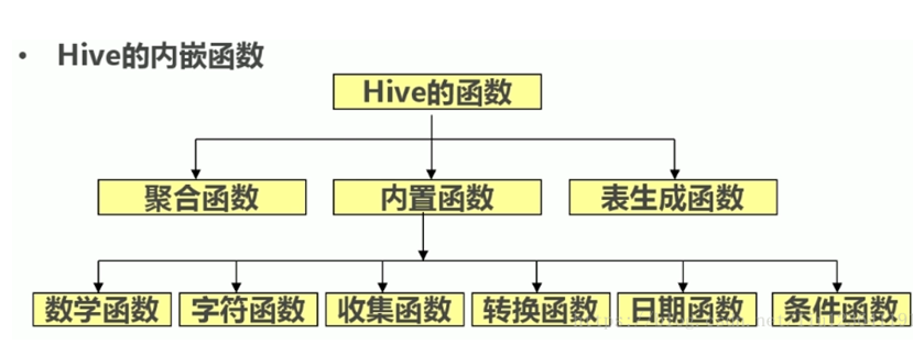
1. System built-in function
(1)Relational operation (point me)
(2)Logical operation (point I)
(3) Mathematical operation
- • addition operation:+
- • subtraction:-
- • multiplication operation:*
- • division operation:/
- • residual operation:%
- • bit and operation:&
- • bit or operation:|
- • bitwise exclusive or operation:^
- • bit reversal operation:~
create table dual(id string);
Prepare text with only one space to put into the table
select 1 + 9 from dual;
(4) Numerical operation
- Rounding function: round
- Specify precision rounding function: round
- Rounding down function: floor
- Rounding up function: ceil
- Rounding up function: ceiling
- Random number function: rand
- Natural exponential function: exp
- Base 10 logarithm function: log10
- Base 2 logarithmic function: log2
- Log function: log
- Power operation function: pow
- power operation function: power
- Square function: sqrt
- Binary function: bin
- Hex function: hex
- Reverse hex function: unhex
- Binary conversion function: conv
- Absolute value function: abs
- Positive remainder function: pmod
- Sine function: sin
- Inverse sine function: asin
- Cosine function: cos
- Inverse cosine function: acos
- Positive function: positive
- Negative function: negative
- (5) Date function
- UNIX timestamp to date function: from_unixtime
- Get current UNIX timestamp function: unix_timestamp
- Date to UNIX timestamp function: unix_timestamp
- Specified format date to UNIX timestamp function: unix_timestamp
- Date time to date function: to_date
- Date to year function: year
- Date to month function: month
- Date conversion function: day
- Date to hour function: hour
- Date to minute function: minute
- Date to second function: Second
- Date to week function: weekofyear
- Date comparison function: datediff
- Date addition function: date_add
- Date reduction function: date_sub
- (6) String function
- String length function: length
- String inversion function: reverse
- String concatenation function: concat
- Delimited string concatenation function: concat_ws
- String interception function: substr,substring
- String interception function: substr,substring
- String to uppercase function: upper,ucase
- String to lowercase function: lower,lcase
- De whitespace function: trim
- Left space function: ltrim
- Function to remove space on the right: rtrim
- Regular expression replacement function: regexp_replace
- Regular expression parsing function: regexp_extract
- URL parsing function: parse_url
- JSON parsing function: get_json_object
- space string function: space
- Repeat string function: repeat
- First character function: ascii
- Left complement function: lpad
- Right complement function: rpad
- Split string function: split
- Collection lookup function: find_in_set
get_json_object
Syntax: get_json_object(string json_string, string path)
Return value: string
Description: parse json string_ String to return the content specified by path. NULL is returned if the json string entered is invalid.
select  get_json_object('
	{"store":
		{"fruit":[
			{"weight":8,"type":"apple"},
			{"weight":9,"type":"pear"}
			],
		"bicycle":{"price":19.95,"color":"red"}
	},
	"email":"amy@only_for_json_udf_test.net",
	"owner":"amy"
	}'
,'$.store.fruit.type[0]');
2. Common built-in functions
(1) Empty field assignment
NVL: assign a value to the data whose value is NULL. Its format is NVL (value, default_value). Its function is to return default if value is NULL_ Value, otherwise return the value of value. If both parameters are NULL, return NULL.
--If the comm of the employee is NULL, use - 1 instead
select comm,nvl(comm, -1) from emp;
--If the comm of the employee is NULL, the leader id is used instead
select comm, nvl(comm,mgr) from emp;
(2) Conditional function
a.If function: if
Syntax: if (Boolean TestCondition, t ValueTrue, t valuefalse or null)
Return value: T
Description: when the condition testCondition is TRUE, valueTrue is returned; Otherwise, valuefalse ornull is returned
select if(1=2,100,200) from dual;
200
select if(1=1,100,200) from dual;
100
b. Non empty lookup function: coalesce
Syntax: coalesce(T v1, T v2,...)
Return value: T
Description: returns the first non null value in the parameter; Returns NULL if all values are null
select coalesce(null,'100','50') from dual;
100
c. Conditional judgment function: case
Syntax: case a when b then c [when d then e]... [else f] end
Return value: T
Note: if a equals b, c is returned; If a equals d, then e is returned;
Otherwise, return f
select
case 100
when 50 then 'tom'
when 100 then 'mary'
else 'tim'
end ;
mary
(3) Row to column (multi row to single column)
a.concat(string a/col, string b/col...):
Returns the connected result of the input string, and supports any input string;
--Splice string "---" ">
select concat("---",">");
select concat(ename,job) from emp;
b.concat_ws(separator, str1, str2,...):
It is a special form of concat(). The separator between the first parameter and the remaining parameters. The delimiter can be the same string as the remaining parameters. If the delimiter is NULL, the return value will also be NULL. This function skips any NULL and empty strings after the delimiter parameter. The separator will be added between the connected strings;
--Splice string~_^
select concat_ws("_","~","^");
d.collect_set(col):
The function only accepts basic data types. Its main function is to de summarize the values of a field and generate an array type field.
select concat_ws('-',collect_set(job)) from emp;
--Count the employees with the same salary in each department

select concat(deptno,'-',sal)  base ,ename from emp;

+------------+--------------+
|   t.base   |     name     |
+------------+--------------+
| 10-1300.0  | MILLER       |
| 10-2450.0  | CLARK        |
| 10-5000.0  | KING         |
| 20-1100.0  | ADAMS        |
| 20-2975.0  | JONES        |
| 20-3000.0  | SCOTT|FORD   |
| 20-800.0   | SMITH        |
| 30-1250.0  | WARD|MARTIN  |
| 30-1500.0  | TURNER       |
| 30-1600.0  | ALLEN        |
| 30-2850.0  | BLAKE        |
| 30-950.0   | JAMES        |
| 50-1200.0  | TOM          |
+------------+--------------+

--First connect the department number with the salary
select concat(deptno,'-',sal)  base ,ename from emp;
+------------+---------+
|    base    |  ename  |
+------------+---------+
| 20-800.0   | SMITH   |
| 30-1600.0  | ALLEN   |
| 30-1250.0  | WARD    |
| 20-2975.0  | JONES   |
| 30-1250.0  | MARTIN  |
| 30-2850.0  | BLAKE   |
| 10-2450.0  | CLARK   |
| 20-3000.0  | SCOTT   |
| 10-5000.0  | KING    |
| 30-1500.0  | TURNER  |
| 20-1100.0  | ADAMS   |
| 30-950.0   | JAMES   |
| 20-3000.0  | FORD    |
| 10-1300.0  | MILLER  |
| 50-1200.0  | TOM     |
+------------+---------+
-- Continue to process the results of the previous step according to base Group aggregation,

select t.base,collect_set(t.ename)
from (select concat(deptno,'-',sal)  base ,ename from emp)t
group by t.base;

+------------+--------------------+
|   t.base   |        _c1         |
+------------+--------------------+
| 10-2450.0  | ["CLARK"]          |
| 10-5000.0  | ["KING"]           |
| 20-3000.0  | ["SCOTT","FORD"]   |
| 30-1250.0  | ["WARD","MARTIN"]  |
| 30-1500.0  | ["TURNER"]         |
| 30-2850.0  | ["BLAKE"]          |
| 50-1200.0  | ["TOM"]            |
| 10-1300.0  | ["MILLER"]         |
| 20-1100.0  | ["ADAMS"]          |
| 20-2975.0  | ["JONES"]          |
| 20-800.0   | ["SMITH"]          |
| 30-1600.0  | ["ALLEN"]          |
| 30-950.0   | ["JAMES"]          |
+------------+--------------------+
-- Process the results of the previous step again
select t.base,concat_ws('|',collect_set(t.ename))
from (select concat(deptno,'-',sal)  base ,ename from emp)t
group by t.base;
Idea:
- Splice the department number and salary together
select concat(deptno,"-",sal) base,ename from emp;
- Group by department number + salary
select t.base, collect_set(t.ename) name
from (select concat(deptno,"-",sal) base,ename from emp) t
group by t.base;
- Multiple employees need to be spliced together
select t.base, concat_ws('|',collect_set(t.ename)) name
from (select concat(deptno,"-",sal) base,ename from emp) t
group by t.base;
(4) Column to row
a.explode
- The expand function can expand an array or map type field,
Expand (array) causes each element in the array list to generate a row in the result; Expand (map) makes each pair of elements in the map as a row, key as a column and value as a column in the result.
- In general, expand can be used directly or combined with lateral view as needed
select explode(array("hadoop","spark","flink"));
b.lateral view
- Usage: lateral view udtf(expression) tablealias as columnalias
- Explanation: it is used with split, expand and other udtf s. It can split a column of data into multiple rows of data. On this basis, the split data can be aggregated.
Prepare data:
create  table p1(name string,children array<string>,address Map<string,string>)
row format delimited fields terminated by '|'
collection items terminated by ','
map keys terminated by ':';

vim maparray.txt
zhangsan|child1,child2,child3,child4|k1:v1,k2:v2
lisi|child5,child6,child7,child8|k3:v3,k4:v4

load data local inpath '/home/offcn/tmp/maparray.txt' into table p1;

select * from p1;
+-----------+----------------------------------------+------------------------+
|  p1.name  |              p1.children               |       p1.address       |
+-----------+----------------------------------------+------------------------+
| zhangsan  | ["child1","child2","child3","child4"]  | {"k1":"v1","k2":"v2"}  |
| lisi      | ["child5","child6","child7","child8"]  | {"k3":"v3","k4":"v4"}  |
+-----------+----------------------------------------+------------------------+

select explode(children) as myChild from p1;
select explode(address) as (myMapKey, myMapValue) from p1;

--If you want to splice and combine the original table and split columns
select p1.*,childrenView.*,addressView.* from p1
lateral view explode(children) childrenView as myChild
lateral view explode(address) addressView as myMapKey, myMapValue;

+-----------+----------------------------------------+------------------------+-----------------------+-----------------------+-------------------------+
|  p1.name  |              p1.children               |       p1.address       | childrenview.mychild  | addressview.mymapkey  | addressview.mymapvalue  |
+-----------+----------------------------------------+------------------------+-----------------------+-----------------------+-------------------------+
| zhangsan  | ["child1","child2","child3","child4"]  | {"k1":"v1","k2":"v2"}  | child1                | k1                    | v1                      |
| zhangsan  | ["child1","child2","child3","child4"]  | {"k1":"v1","k2":"v2"}  | child1                | k2                    | v2                      |
| zhangsan  | ["child1","child2","child3","child4"]  | {"k1":"v1","k2":"v2"}  | child2                | k1                    | v1                      |
| zhangsan  | ["child1","child2","child3","child4"]  | {"k1":"v1","k2":"v2"}  | child2                | k2                    | v2                      |
| zhangsan  | ["child1","child2","child3","child4"]  | {"k1":"v1","k2":"v2"}  | child3                | k1                    | v1                      |
| zhangsan  | ["child1","child2","child3","child4"]  | {"k1":"v1","k2":"v2"}  | child3                | k2                    | v2                      |
| zhangsan  | ["child1","child2","child3","child4"]  | {"k1":"v1","k2":"v2"}  | child4                | k1                    | v1                      |
| zhangsan  | ["child1","child2","child3","child4"]  | {"k1":"v1","k2":"v2"}  | child4                | k2                    | v2                      |
| lisi      | ["child5","child6","child7","child8"]  | {"k3":"v3","k4":"v4"}  | child5                | k3                    | v3                      |
| lisi      | ["child5","child6","child7","child8"]  | {"k3":"v3","k4":"v4"}  | child5                | k4                    | v4                      |
| lisi      | ["child5","child6","child7","child8"]  | {"k3":"v3","k4":"v4"}  | child6                | k3                    | v3                      |
| lisi      | ["child5","child6","child7","child8"]  | {"k3":"v3","k4":"v4"}  | child6                | k4                    | v4                      |
| lisi      | ["child5","child6","child7","child8"]  | {"k3":"v3","k4":"v4"}  | child7                | k3                    | v3                      |
| lisi      | ["child5","child6","child7","child8"]  | {"k3":"v3","k4":"v4"}  | child7                | k4                    | v4                      |
| lisi      | ["child5","child6","child7","child8"]  | {"k3":"v3","k4":"v4"}  | child8                | k3                    | v3                      |
| lisi      | ["child5","child6","child7","child8"]  | {"k3":"v3","k4":"v4"}  | child8                | k4                    | v4                      |
+-----------+----------------------------------------+------------------------+-----------------------+-----------------------+-------------------------+
(5) Window function (windowing function)
The window function in hive is similar to the window function in sql. It is used to do some data analysis. It is generally used for olap analysis (online analysis and processing). Most window functions are aimed at the internal processing of partitions (Windows). Hive and oracle provide window opening functions, which are not provided before MySQL 8.0, but MySQL 8.0 supports two important functions: window function (over) and common table expression (with)!
Syntax structure:
Window function over (partition by column name, column name... order by column name, rows between start position and end position)
explain:
- over() function:
The over() function includes three functions: partition by column name, sorting order by column name, and specifying the start position and end position of the window range rows between. It determines the aggregation range of the aggregation function. By default, it aggregates the data in the whole window. The aggregation function calls each piece of data once
- partition by clause:
Use the partition by clause to partition the data. You can use partition by to aggregate the data in the area. You can follow multiple fields, (partition by.. order by) can be replaced by (distribute by.. sort by..).
- order by clause:
order by means sorting. It means sorting according to the specified field in the window. Only one field can be followed.
- rows between :
rows between start position and end position, window size limit:
-
- following: back
- Current row: current row
- unbounded: starting point (generally used in combination with preceding and following)
- unbounded preceding: indicates the front row (starting point) of the window
- unbounded following: indicates the last line (end point) of the window
Prepare data:
create table t2(ip string, createtime string, url string,pvs int)
row format delimited fields terminated by ',';


vim t2.txt
192.168.233.11,2021-04-10,url2,5
192.168.233.11,2021-04-12,url1,4
192.168.233.11,2021-04-10,1url3,5
192.168.233.11,2021-04-11,url6,3
192.168.233.11,2021-04-13,url4,6
192.168.233.12,2021-04-10,url7,5
192.168.233.12,2021-04-11,url4,1
192.168.233.12,2021-04-10,url5,5
192.168.233.13,2021-04-11,url22,3
192.168.233.13,2021-04-10,url11,11
192.168.233.13,2021-04-12,1url33,7
192.168.233.14,2021-04-13,url66,9
192.168.233.14,2021-04-12,url77,1
192.168.233.14,2021-04-13,url44,12
192.168.233.14,2021-04-11,url55,33

load data local inpath "/home/offcn/tmp/t2.txt" into table t2;
select * from t2;
a. Window aggregate function
Solve the problem of statistics within groups and displaying non group fields
- count windowing function
--Count each ip,Number and details of data in each time period
select ip,createtime,count(pvs)
from t2
group by ip,createtime;

+-----------------+-------------+------+
|       ip        | createtime  | _c2  |
+-----------------+-------------+------+
| 192.168.233.11  | 2021-04-10  | 2    |
| 192.168.233.11  | 2021-04-11  | 1    |
| 192.168.233.11  | 2021-04-12  | 1    |
| 192.168.233.11  | 2021-04-13  | 1    |
| 192.168.233.12  | 2021-04-10  | 2    |
| 192.168.233.12  | 2021-04-11  | 1    |
| 192.168.233.13  | 2021-04-10  | 1    |
| 192.168.233.13  | 2021-04-11  | 1    |
| 192.168.233.13  | 2021-04-12  | 1    |
| 192.168.233.14  | 2021-04-11  | 1    |
| 192.168.233.14  | 2021-04-12  | 1    |
| 192.168.233.14  | 2021-04-13  | 2    |
+-----------------+-------------+------+

Problem: Discovery group by The detailed data cannot be displayed after. At this time, you need to use the window function
select ip,createtime,url,pvs,count(pvs) over(partition by ip,createtime)
from t2;

+-----------------+-------------+---------+------+-----------------+
|       ip        | createtime  |   url   | pvs  | count_window_0  |
+-----------------+-------------+---------+------+-----------------+
| 192.168.233.11  | 2021-04-10  | url2    | 5    | 2               |
| 192.168.233.11  | 2021-04-10  | 1url3   | 5    | 2               |
| 192.168.233.11  | 2021-04-11  | url6    | 3    | 1               |
| 192.168.233.11  | 2021-04-12  | url1    | 4    | 1               |
| 192.168.233.11  | 2021-04-13  | url4    | 6    | 1               |
| 192.168.233.12  | 2021-04-10  | url5    | 5    | 2               |
| 192.168.233.12  | 2021-04-10  | url7    | 5    | 2               |
| 192.168.233.12  | 2021-04-11  | url4    | 1    | 1               |
| 192.168.233.13  | 2021-04-10  | url11   | 11   | 1               |
| 192.168.233.13  | 2021-04-11  | url22   | 3    | 1               |
| 192.168.233.13  | 2021-04-12  | 1url33  | 7    | 1               |
| 192.168.233.14  | 2021-04-11  | url55   | 33   | 1               |
| 192.168.233.14  | 2021-04-12  | url77   | 1    | 1               |
| 192.168.233.14  | 2021-04-13  | url66   | 9    | 2               |
| 192.168.233.14  | 2021-04-13  | url44   | 12   | 2               |
+-----------------+-------------+---------+------+-----------------+
- sum windowing function
--Count the total pv number and details of each ip and each time period
select ip,createtime,url,pvs,sum(pvs) over(partition by ip,createtime)
from t2;
- avg windowing function
--Count the draw pv times and details of each ip and each time period
select ip,createtime, url,pvs,avg(pvs) over(partition by ip,createtime)
from t2;
- min windowing function
--Count the minimum pv number and details of each ip and each time period
select ip,createtime, url,pvs,min(pvs) over(partition by ip,createtime)
from t2;
- max windowing function
--Count the maximum pv number and details of each ip and each time period
select ip,createtime, url,pvs,max(pvs) over(partition by ip,createtime)
from t2;
- Window control statement
select  *,
--All rows in the group
--according to ip grouping
sum(pvs) over(partition by ip) AS c_1 ,
--according to createtime Group and display in ascending order according to the field
sum(pvs) over(order  by createtime) AS c_2 ,
--The default is from the starting point to the current line,
sum(pvs) over(partition by ip order by createtime asc) AS c_3,
--From the starting point to the current line, the result is the same as sales_3 Different. According to the sorting order, the results may accumulate differently
sum(pvs) over(partition by ip order by createtime asc rows between unbounded preceding and current row) AS c_4,
--Current row+3 lines ahead
sum(pvs) over(partition by ip order by createtime asc rows between 3 preceding and current row) AS c_5,
--Current row+3 lines ahead+1 line back
sum(pvs) over(partition by ip order by createtime asc rows between 3 preceding and 1 following) AS c_6,
--Current row+All lines back
sum(pvs) over(partition by ip order by createtime asc rows between current row and unbounded following) AS c_7
from t2;

--according to ip Grouping, all rows in the grouping are accumulated
select  *,
sum(pvs) over(partition by ip) AS c_1
from t2;

+-----------------+----------------+---------+---------+------+
|      t2.ip      | t2.createtime  | t2.url  | t2.pvs  | c_1  |
+-----------------+----------------+---------+---------+------+
| 192.168.233.11  | 2021-04-10     | url2    | 5       | 23   |
| 192.168.233.11  | 2021-04-12     | url1    | 4       | 23   |
| 192.168.233.11  | 2021-04-10     | 1url3   | 5       | 23   |
| 192.168.233.11  | 2021-04-11     | url6    | 3       | 23   |
| 192.168.233.11  | 2021-04-13     | url4    | 6       | 23   |
| 192.168.233.12  | 2021-04-10     | url5    | 5       | 11   |
| 192.168.233.12  | 2021-04-11     | url4    | 1       | 11   |
| 192.168.233.12  | 2021-04-10     | url7    | 5       | 11   |
| 192.168.233.13  | 2021-04-12     | 1url33  | 7       | 21   |
| 192.168.233.13  | 2021-04-11     | url22   | 3       | 21   |
| 192.168.233.13  | 2021-04-10     | url11   | 11      | 21   |
| 192.168.233.14  | 2021-04-13     | url44   | 12      | 55   |
| 192.168.233.14  | 2021-04-11     | url55   | 33      | 55   |
| 192.168.233.14  | 2021-04-13     | url66   | 9       | 55   |
| 192.168.233.14  | 2021-04-12     | url77   | 1       | 55   |
+-----------------+----------------+---------+---------+------+

-- Sort by time, group by time, and accumulate the same time one by one
select  *,
sum(pvs) over(order  by createtime) AS c_2
from t2;

+-----------------+----------------+---------+---------+------+
|      t2.ip      | t2.createtime  | t2.url  | t2.pvs  | c_2  |
+-----------------+----------------+---------+---------+------+
| 192.168.233.11  | 2021-04-10     | url2    | 5       | 31   |
| 192.168.233.13  | 2021-04-10     | url11   | 11      | 31   |
| 192.168.233.12  | 2021-04-10     | url5    | 5       | 31   |
| 192.168.233.12  | 2021-04-10     | url7    | 5       | 31   |
| 192.168.233.11  | 2021-04-10     | 1url3   | 5       | 31   |
| 192.168.233.11  | 2021-04-11     | url6    | 3       | 71   |
| 192.168.233.13  | 2021-04-11     | url22   | 3       | 71   |
| 192.168.233.14  | 2021-04-11     | url55   | 33      | 71   |
| 192.168.233.12  | 2021-04-11     | url4    | 1       | 71   |
| 192.168.233.11  | 2021-04-12     | url1    | 4       | 83   |
| 192.168.233.14  | 2021-04-12     | url77   | 1       | 83   |
| 192.168.233.13  | 2021-04-12     | 1url33  | 7       | 83   |
| 192.168.233.11  | 2021-04-13     | url4    | 6       | 110  |
| 192.168.233.14  | 2021-04-13     | url44   | 12      | 110  |
| 192.168.233.14  | 2021-04-13     | url66   | 9       | 110  |
+-----------------+----------------+---------+---------+------+

-- according to ip Divide into large groups, and then divide into groups according to the chronological order within the group, and accumulate one by one within the large group
select  *,
sum(pvs) over(partition by ip order by createtime asc) AS c_3
from t2;

+-----------------+----------------+---------+---------+------+
|      t2.ip      | t2.createtime  | t2.url  | t2.pvs  | c_3  |
+-----------------+----------------+---------+---------+------+
| 192.168.233.11  | 2021-04-10     | url2    | 5       | 10   |
| 192.168.233.11  | 2021-04-10     | 1url3   | 5       | 10   |
| 192.168.233.11  | 2021-04-11     | url6    | 3       | 13   |
| 192.168.233.11  | 2021-04-12     | url1    | 4       | 17   |
| 192.168.233.11  | 2021-04-13     | url4    | 6       | 23   |
| 192.168.233.12  | 2021-04-10     | url5    | 5       | 10   |
| 192.168.233.12  | 2021-04-10     | url7    | 5       | 10   |
| 192.168.233.12  | 2021-04-11     | url4    | 1       | 11   |
| 192.168.233.13  | 2021-04-10     | url11   | 11      | 11   |
| 192.168.233.13  | 2021-04-11     | url22   | 3       | 14   |
| 192.168.233.13  | 2021-04-12     | 1url33  | 7       | 21   |
| 192.168.233.14  | 2021-04-11     | url55   | 33      | 33   |
| 192.168.233.14  | 2021-04-12     | url77   | 1       | 34   |
| 192.168.233.14  | 2021-04-13     | url66   | 9       | 55   |
| 192.168.233.14  | 2021-04-13     | url44   | 12      | 55   |
+-----------------+----------------+---------+---------+------+


-- according to ip Divide into large groups according to time url Sort and divide into groups, and accumulate one by one in the large group

select  *,
sum(pvs) over(partition by ip order by createtime asc,url) AS c_3
from t2;

+-----------------+----------------+---------+---------+------+
|      t2.ip      | t2.createtime  | t2.url  | t2.pvs  | c_3  |
+-----------------+----------------+---------+---------+------+
| 192.168.233.11  | 2021-04-10     | 1url3   | 5       | 5    |
| 192.168.233.11  | 2021-04-10     | url2    | 5       | 10   |
| 192.168.233.11  | 2021-04-11     | url6    | 3       | 13   |
| 192.168.233.11  | 2021-04-12     | url1    | 4       | 17   |
| 192.168.233.11  | 2021-04-13     | url4    | 6       | 23   |
| 192.168.233.12  | 2021-04-10     | url5    | 5       | 5    |
| 192.168.233.12  | 2021-04-10     | url7    | 5       | 10   |
| 192.168.233.12  | 2021-04-11     | url4    | 1       | 11   |
| 192.168.233.13  | 2021-04-10     | url11   | 11      | 11   |
| 192.168.233.13  | 2021-04-11     | url22   | 3       | 14   |
| 192.168.233.13  | 2021-04-12     | 1url33  | 7       | 21   |
| 192.168.233.14  | 2021-04-11     | url55   | 33      | 33   |
| 192.168.233.14  | 2021-04-12     | url77   | 1       | 34   |
| 192.168.233.14  | 2021-04-13     | url44   | 12      | 46   |
| 192.168.233.14  | 2021-04-13     | url66   | 9       | 55   |
+-----------------+----------------+---------+---------+------+


-- according to ip It is divided into windows. The current line and all previous lines of the current window are accumulated in ascending order of time(default)
select  *,
sum(pvs) over(partition by ip order by createtime asc rows between unbounded preceding and current row) AS c_4
from t2;

+-----------------+----------------+---------+---------+------+
|      t2.ip      | t2.createtime  | t2.url  | t2.pvs  | c_4  |
+-----------------+----------------+---------+---------+------+
| 192.168.233.11  | 2021-04-10     | url2    | 5       | 5    |
| 192.168.233.11  | 2021-04-10     | 1url3   | 5       | 10   |
| 192.168.233.11  | 2021-04-11     | url6    | 3       | 13   |
| 192.168.233.11  | 2021-04-12     | url1    | 4       | 17   |
| 192.168.233.11  | 2021-04-13     | url4    | 6       | 23   |
| 192.168.233.12  | 2021-04-10     | url5    | 5       | 5    |
| 192.168.233.12  | 2021-04-10     | url7    | 5       | 10   |
| 192.168.233.12  | 2021-04-11     | url4    | 1       | 11   |
| 192.168.233.13  | 2021-04-10     | url11   | 11      | 11   |
| 192.168.233.13  | 2021-04-11     | url22   | 3       | 14   |
| 192.168.233.13  | 2021-04-12     | 1url33  | 7       | 21   |
| 192.168.233.14  | 2021-04-11     | url55   | 33      | 33   |
| 192.168.233.14  | 2021-04-12     | url77   | 1       | 34   |
| 192.168.233.14  | 2021-04-13     | url66   | 9       | 43   |
| 192.168.233.14  | 2021-04-13     | url44   | 12      | 55   |
+-----------------+----------------+---------+---------+------+

-- according to ip Divided into windows, the current line and the first 3 lines (4 lines in total) of the current window are accumulated in ascending time order
select  *,
sum(pvs) over(partition by ip order by createtime asc rows between 3 preceding and current row) AS c_5
from t2;

+-----------------+----------------+---------+---------+------+
|      t2.ip      | t2.createtime  | t2.url  | t2.pvs  | c_5  |
+-----------------+----------------+---------+---------+------+
| 192.168.233.11  | 2021-04-10     | url2    | 5       | 5    |
| 192.168.233.11  | 2021-04-10     | 1url3   | 5       | 10   |
| 192.168.233.11  | 2021-04-11     | url6    | 3       | 13   |
| 192.168.233.11  | 2021-04-12     | url1    | 4       | 17   |
| 192.168.233.11  | 2021-04-13     | url4    | 6       | 18   |
| 192.168.233.12  | 2021-04-10     | url5    | 5       | 5    |
| 192.168.233.12  | 2021-04-10     | url7    | 5       | 10   |
| 192.168.233.12  | 2021-04-11     | url4    | 1       | 11   |
| 192.168.233.13  | 2021-04-10     | url11   | 11      | 11   |
| 192.168.233.13  | 2021-04-11     | url22   | 3       | 14   |
| 192.168.233.13  | 2021-04-12     | 1url33  | 7       | 21   |
| 192.168.233.14  | 2021-04-11     | url55   | 33      | 33   |
| 192.168.233.14  | 2021-04-12     | url77   | 1       | 34   |
| 192.168.233.14  | 2021-04-13     | url66   | 9       | 43   |
| 192.168.233.14  | 2021-04-13     | url44   | 12      | 55   |
+-----------------+----------------+---------+---------+------+

-- according to ip It is divided into windows. The current line, the first three lines and the next line of the current line of the current window are accumulated in ascending time order
select  *,
sum(pvs) over(partition by ip order by createtime asc rows between 3 preceding and 1 following) AS c_6
from t2;

+-----------------+----------------+---------+---------+-------+
|      t2.ip      | t2.createtime  | t2.url  | t2.pvs  | c_6  |
+-----------------+----------------+---------+---------+-------+
| 192.168.233.11  | 2021-04-10     | url2    | 5       | 10    |
| 192.168.233.11  | 2021-04-10     | 1url3   | 5       | 13    |
| 192.168.233.11  | 2021-04-11     | url6    | 3       | 17    |
| 192.168.233.11  | 2021-04-12     | url1    | 4       | 23    |
| 192.168.233.11  | 2021-04-13     | url4    | 6       | 18    |
| 192.168.233.12  | 2021-04-10     | url5    | 5       | 10    |
| 192.168.233.12  | 2021-04-10     | url7    | 5       | 11    |
| 192.168.233.12  | 2021-04-11     | url4    | 1       | 11    |
| 192.168.233.13  | 2021-04-10     | url11   | 11      | 14    |
| 192.168.233.13  | 2021-04-11     | url22   | 3       | 21    |
| 192.168.233.13  | 2021-04-12     | 1url33  | 7       | 21    |
| 192.168.233.14  | 2021-04-11     | url55   | 33      | 34    |
| 192.168.233.14  | 2021-04-12     | url77   | 1       | 43    |
| 192.168.233.14  | 2021-04-13     | url66   | 9       | 55    |
| 192.168.233.14  | 2021-04-13     | url44   | 12      | 55    |
+-----------------+----------------+---------+---------+-------+

-- according to ip It is divided into windows. The window starts from the current line of the current window and accumulates to the last line of the window in ascending time order
select  *,
sum(pvs) over(partition by ip order by createtime asc rows between current row and unbounded following) AS c_7
from t2;
+-----------------+----------------+---------+---------+------+
|      t2.ip      | t2.createtime  | t2.url  | t2.pvs  | c_7  |
+-----------------+----------------+---------+---------+------+
| 192.168.233.11  | 2021-04-10     | url2    | 5       | 23   |
| 192.168.233.11  | 2021-04-10     | 1url3   | 5       | 18   |
| 192.168.233.11  | 2021-04-11     | url6    | 3       | 13   |
| 192.168.233.11  | 2021-04-12     | url1    | 4       | 10   |
| 192.168.233.11  | 2021-04-13     | url4    | 6       | 6    |
| 192.168.233.12  | 2021-04-10     | url5    | 5       | 11   |
| 192.168.233.12  | 2021-04-10     | url7    | 5       | 6    |
| 192.168.233.12  | 2021-04-11     | url4    | 1       | 1    |
| 192.168.233.13  | 2021-04-10     | url11   | 11      | 21   |
| 192.168.233.13  | 2021-04-11     | url22   | 3       | 10   |
| 192.168.233.13  | 2021-04-12     | 1url33  | 7       | 7    |
| 192.168.233.14  | 2021-04-11     | url55   | 33      | 55   |
| 192.168.233.14  | 2021-04-12     | url77   | 1       | 22   |
| 192.168.233.14  | 2021-04-13     | url66   | 9       | 21   |
| 192.168.233.14  | 2021-04-13     | url44   | 12      | 12   |
+-----------------+----------------+---------+---------+------+
b. Window analysis function
Solving cascading problems
- first_value windowing function
Count each ip Heben ip The first time I entered the website pv Difference and detailed data

according to ip Grouping: the group is sorted in ascending time order, and the first one in the group is selected
select *,first_value(pvs) over(partition by ip order by createtime) haha
from t2;
+-----------------+----------------+---------+---------+-------+
|      t2.ip      | t2.createtime  | t2.url  | t2.pvs  | haha  |
+-----------------+----------------+---------+---------+-------+
| 192.168.233.11  | 2021-04-10     | url2    | 5       | 5     |
| 192.168.233.11  | 2021-04-10     | 1url3   | 5       | 5     |
| 192.168.233.11  | 2021-04-11     | url6    | 3       | 5     |
| 192.168.233.11  | 2021-04-12     | url1    | 4       | 5     |
| 192.168.233.11  | 2021-04-13     | url4    | 6       | 5     |
| 192.168.233.12  | 2021-04-10     | url5    | 5       | 5     |
| 192.168.233.12  | 2021-04-10     | url7    | 5       | 5     |
| 192.168.233.12  | 2021-04-11     | url4    | 1       | 5     |
| 192.168.233.13  | 2021-04-10     | url11   | 11      | 11    |
| 192.168.233.13  | 2021-04-11     | url22   | 3       | 11    |
| 192.168.233.13  | 2021-04-12     | 1url33  | 7       | 11    |
| 192.168.233.14  | 2021-04-11     | url55   | 33      | 33    |
| 192.168.233.14  | 2021-04-12     | url77   | 1       | 33    |
| 192.168.233.14  | 2021-04-13     | url66   | 9       | 33    |
| 192.168.233.14  | 2021-04-13     | url44   | 12      | 33    |
+-----------------+----------------+---------+---------+-------+


with aaa as(
select *,first_value(pvs) over(partition by ip order by createtime) haha
from t2)
select *,(aaa.pvs-aaa.haha) from aaa;

+-----------------+-----------------+----------+----------+-----------+------+
|     aaa.ip      | aaa.createtime  | aaa.url  | aaa.pvs  | aaa.haha  | _c1  |
+-----------------+-----------------+----------+----------+-----------+------+
| 192.168.233.11  | 2021-04-10      | url2     | 5        | 5         | 0    |
| 192.168.233.11  | 2021-04-10      | 1url3    | 5        | 5         | 0    |
| 192.168.233.11  | 2021-04-11      | url6     | 3        | 5         | -2   |
| 192.168.233.11  | 2021-04-12      | url1     | 4        | 5         | -1   |
| 192.168.233.11  | 2021-04-13      | url4     | 6        | 5         | 1    |
| 192.168.233.12  | 2021-04-10      | url5     | 5        | 5         | 0    |
| 192.168.233.12  | 2021-04-10      | url7     | 5        | 5         | 0    |
| 192.168.233.12  | 2021-04-11      | url4     | 1        | 5         | -4   |
| 192.168.233.13  | 2021-04-10      | url11    | 11       | 11        | 0    |
| 192.168.233.13  | 2021-04-11      | url22    | 3        | 11        | -8   |
| 192.168.233.13  | 2021-04-12      | 1url33   | 7        | 11        | -4   |
| 192.168.233.14  | 2021-04-11      | url55    | 33       | 33        | 0    |
| 192.168.233.14  | 2021-04-12      | url77    | 1        | 33        | -32  |
| 192.168.233.14  | 2021-04-13      | url66    | 9        | 33        | -24  |
| 192.168.233.14  | 2021-04-13      | url44    | 12       | 33        | -21  |
+-----------------+-----------------+----------+----------+-----------+------+


with as sentence:
with...as...Also known as the subquery part,Statement allow hive Define a sql fragment,For the whole sql use
- last_value windowing function
First according to ip Group, and then slide the window according to the sort field(In other words ip And sort fields determine the window) Count each ip,Each time period and this ip,Last access to the website in this time period pv Difference and detailed data select *,last_value(pvs) over(partition by ip order by createtime) haha from t2; +-----------------+----------------+---------+---------+-------+ | t2.ip | t2.createtime | t2.url | t2.pvs | haha | +-----------------+----------------+---------+---------+-------+ | 192.168.233.11 | 2021-04-10 | url2 | 5 | 5 | | 192.168.233.11 | 2021-04-10 | 1url3 | 5 | 5 | | 192.168.233.11 | 2021-04-11 | url6 | 3 | 3 | | 192.168.233.11 | 2021-04-12 | url1 | 4 | 4 | | 192.168.233.11 | 2021-04-13 | url4 | 6 | 6 | | 192.168.233.12 | 2021-04-10 | url5 | 5 | 5 | | 192.168.233.12 | 2021-04-10 | url7 | 5 | 5 | | 192.168.233.12 | 2021-04-11 | url4 | 1 | 1 | | 192.168.233.13 | 2021-04-10 | url11 | 11 | 11 | | 192.168.233.13 | 2021-04-11 | url22 | 3 | 3 | | 192.168.233.13 | 2021-04-12 | 1url33 | 7 | 7 | | 192.168.233.14 | 2021-04-11 | url55 | 33 | 33 | | 192.168.233.14 | 2021-04-12 | url77 | 1 | 1 | | 192.168.233.14 | 2021-04-13 | url66 | 9 | 12 | | 192.168.233.14 | 2021-04-13 | url44 | 12 | 12 | +-----------------+----------------+---------+---------+-------+ with aaa as( select *,last_value(pvs) over(partition by ip order by createtime) haha from t2) select *,(aaa.pvs-aaa.haha) from aaa; +-----------------+-----------------+----------+----------+-----------+------+ | aaa.ip | aaa.createtime | aaa.url | aaa.pvs | aaa.haha | _c1 | +-----------------+-----------------+----------+----------+-----------+------+ | 192.168.233.11 | 2021-04-10 | url2 | 5 | 5 | 0 | | 192.168.233.11 | 2021-04-10 | 1url3 | 5 | 5 | 0 | | 192.168.233.11 | 2021-04-11 | url6 | 3 | 3 | 0 | | 192.168.233.11 | 2021-04-12 | url1 | 4 | 4 | 0 | | 192.168.233.11 | 2021-04-13 | url4 | 6 | 6 | 0 | | 192.168.233.12 | 2021-04-10 | url5 | 5 | 5 | 0 | | 192.168.233.12 | 2021-04-10 | url7 | 5 | 5 | 0 | | 192.168.233.12 | 2021-04-11 | url4 | 1 | 1 | 0 | | 192.168.233.13 | 2021-04-10 | url11 | 11 | 11 | 0 | | 192.168.233.13 | 2021-04-11 | url22 | 3 | 3 | 0 | | 192.168.233.13 | 2021-04-12 | 1url33 | 7 | 7 | 0 | | 192.168.233.14 | 2021-04-11 | url55 | 33 | 33 | 0 | | 192.168.233.14 | 2021-04-12 | url77 | 1 | 1 | 0 | | 192.168.233.14 | 2021-04-13 | url66 | 9 | 12 | -3 | | 192.168.233.14 | 2021-04-13 | url44 | 12 | 12 | 0 | +-----------------+-----------------+----------+----------+-----------+------+ lag Windowing function LAG(col,n,DEFAULT) It is used to count up the second page in the window n Row value Parameter 1 is the column name, and parameter 2 is the up second column name n Line (optional, the default is 1), and parameter 3 is the default value (when the first row is up) n behavior NULL The default value will be taken. If not specified, otherwise NULL Move window up by createtime Move up 2 lines. If it is empty, use balabala replace select *,lag(createtime,2,'balabala') over(partition by ip order by createtime) tmp from t2; +-----------------+----------------+---------+---------+-------------+ | t2.ip | t2.createtime | t2.url | t2.pvs | tmp | +-----------------+----------------+---------+---------+-------------+ | 192.168.233.11 | 2021-04-10 | url2 | 5 | balabala | | 192.168.233.11 | 2021-04-10 | 1url3 | 5 | balabala | | 192.168.233.11 | 2021-04-11 | url6 | 3 | 2021-04-10 | | 192.168.233.11 | 2021-04-12 | url1 | 4 | 2021-04-10 | | 192.168.233.11 | 2021-04-13 | url4 | 6 | 2021-04-11 | | 192.168.233.12 | 2021-04-10 | url5 | 5 | balabala | | 192.168.233.12 | 2021-04-10 | url7 | 5 | balabala | | 192.168.233.12 | 2021-04-11 | url4 | 1 | 2021-04-10 | | 192.168.233.13 | 2021-04-10 | url11 | 11 | balabala | | 192.168.233.13 | 2021-04-11 | url22 | 3 | balabala | | 192.168.233.13 | 2021-04-12 | 1url33 | 7 | 2021-04-10 | | 192.168.233.14 | 2021-04-11 | url55 | 33 | balabala | | 192.168.233.14 | 2021-04-12 | url77 | 1 | balabala | | 192.168.233.14 | 2021-04-13 | url66 | 9 | 2021-04-11 | | 192.168.233.14 | 2021-04-13 | url44 | 12 | 2021-04-12 | +-----------------+----------------+---------+---------+-------------+
lead windowing function
And LAG contrary
LEAD(col,n,DEFAULT) Used for the next step in the statistics window n Row value
 Parameter 1 is the column name, and parameter 2 is the next column name n Line (optional, the default is 1), and parameter 3 is the default value (when the next line n behavior NULL The default value will be taken. If not specified, otherwise NULL

If the window moves down, it moves one line by default. If not, it returns null
select *,lead(createtime) over(partition by ip order by createtime) tmp
from t2;

+-----------------+----------------+---------+---------+-------------+
|      t2.ip      | t2.createtime  | t2.url  | t2.pvs  |     tmp     |
+-----------------+----------------+---------+---------+-------------+
| 192.168.233.11  | 2021-04-10     | url2    | 5       | 2021-04-10  |
| 192.168.233.11  | 2021-04-10     | 1url3   | 5       | 2021-04-11  |
| 192.168.233.11  | 2021-04-11     | url6    | 3       | 2021-04-12  |
| 192.168.233.11  | 2021-04-12     | url1    | 4       | 2021-04-13  |
| 192.168.233.11  | 2021-04-13     | url4    | 6       | NULL        |
| 192.168.233.12  | 2021-04-10     | url5    | 5       | 2021-04-10  |
| 192.168.233.12  | 2021-04-10     | url7    | 5       | 2021-04-11  |
| 192.168.233.12  | 2021-04-11     | url4    | 1       | NULL        |
| 192.168.233.13  | 2021-04-10     | url11   | 11      | 2021-04-11  |
| 192.168.233.13  | 2021-04-11     | url22   | 3       | 2021-04-12  |
| 192.168.233.13  | 2021-04-12     | 1url33  | 7       | NULL        |
| 192.168.233.14  | 2021-04-11     | url55   | 33      | 2021-04-12  |
| 192.168.233.14  | 2021-04-12     | url77   | 1       | 2021-04-13  |
| 192.168.233.14  | 2021-04-13     | url66   | 9       | 2021-04-13  |
| 192.168.233.14  | 2021-04-13     | url44   | 12      | NULL        |
+-----------------+----------------+---------+---------+-------------+


select *,lead(createtime,1,'haha') over(partition by ip order by createtime) tmp
from t2;

+-----------------+----------------+---------+---------+-------------+
|      t2.ip      | t2.createtime  | t2.url  | t2.pvs  |     tmp     |
+-----------------+----------------+---------+---------+-------------+
| 192.168.233.11  | 2021-04-10     | url2    | 5       | 2021-04-10  |
| 192.168.233.11  | 2021-04-10     | 1url3   | 5       | 2021-04-11  |
| 192.168.233.11  | 2021-04-11     | url6    | 3       | 2021-04-12  |
| 192.168.233.11  | 2021-04-12     | url1    | 4       | 2021-04-13  |
| 192.168.233.11  | 2021-04-13     | url4    | 6       | haha        |
| 192.168.233.12  | 2021-04-10     | url5    | 5       | 2021-04-10  |
| 192.168.233.12  | 2021-04-10     | url7    | 5       | 2021-04-11  |
| 192.168.233.12  | 2021-04-11     | url4    | 1       | haha        |
| 192.168.233.13  | 2021-04-10     | url11   | 11      | 2021-04-11  |
| 192.168.233.13  | 2021-04-11     | url22   | 3       | 2021-04-12  |
| 192.168.233.13  | 2021-04-12     | 1url33  | 7       | haha        |
| 192.168.233.14  | 2021-04-11     | url55   | 33      | 2021-04-12  |
| 192.168.233.14  | 2021-04-12     | url77   | 1       | 2021-04-13  |
| 192.168.233.14  | 2021-04-13     | url66   | 9       | 2021-04-13  |
| 192.168.233.14  | 2021-04-13     | url44   | 12      | haha        |
+-----------------+----------------+---------+---------+-------------+
c. Window sort function
Solve the problem of grouping TopN
- rank windowing function
Generate the ranking of data items in the group. If the ranking is equal, there will be a vacancy in the ranking. The data with the same value can be ranked side by side. When there are two second places, the next is the fourth place
- dense_rank windowing function
Generate the ranking of data items in the group. If the ranking is equal, there will be no vacancy in the ranking. The data with the same value can be ranked side by side. If there are two second places, it will still be followed by the third place
- row_number windowing function
Starting from 1, the sequence of records in the group is generated in order. There are two records in the first place, and row_number() will be sorted and returned
- ntile windowing function
It is used to divide the grouped data into n slices according to the window and order, and return the current slice value
If the slices are not uniform, the distribution of the first slice is increased by default
Usage:
according to ip Group by pvs Sort in ascending order,
select *,
row_number() over(partition by ip order by pvs) row_number,
rank() over(partition by ip order by pvs) rank,
dense_rank() over(partition by ip order by pvs) dense_rank,
ntile(3) over(partition by ip order by pvs) ntile
from t2;

+-----------------+----------------+---------+---------+-------------+-------+-------------+--------+
|      t2.ip      | t2.createtime  | t2.url  | t2.pvs  | row_number  | rank  | dense_rank  | ntile  |
+-----------------+----------------+---------+---------+-------------+-------+-------------+--------+
| 192.168.233.11  | 2021-04-11     | url6    | 3       | 1           | 1     | 1           | 1      |
| 192.168.233.11  | 2021-04-12     | url1    | 4       | 2           | 2     | 2           | 1      |
| 192.168.233.11  | 2021-04-10     | url2    | 5       | 3           | 3     | 3           | 2      |
| 192.168.233.11  | 2021-04-10     | 1url3   | 5       | 4           | 3     | 3           | 2      |
| 192.168.233.11  | 2021-04-13     | url4    | 6       | 5           | 5     | 4           | 3      |
| 192.168.233.12  | 2021-04-11     | url4    | 1       | 1           | 1     | 1           | 1      |
| 192.168.233.12  | 2021-04-10     | url5    | 5       | 2           | 2     | 2           | 2      |
| 192.168.233.12  | 2021-04-10     | url7    | 5       | 3           | 2     | 2           | 3      |
| 192.168.233.13  | 2021-04-11     | url22   | 3       | 1           | 1     | 1           | 1      |
| 192.168.233.13  | 2021-04-12     | 1url33  | 7       | 2           | 2     | 2           | 2      |
| 192.168.233.13  | 2021-04-10     | url11   | 11      | 3           | 3     | 3           | 3      |
| 192.168.233.14  | 2021-04-12     | url77   | 1       | 1           | 1     | 1           | 1      |
| 192.168.233.14  | 2021-04-13     | url66   | 9       | 2           | 2     | 2           | 1      |
| 192.168.233.14  | 2021-04-13     | url44   | 12      | 3           | 3     | 3           | 2      |
| 192.168.233.14  | 2021-04-11     | url55   | 33      | 4           | 4     | 4           | 3      |
+-----------------+----------------+---------+---------+-------------+-------+-------------+--------+

--Count each ip produce pv Top three data( Top3)
with tmp as(
select *,
row_number() over(partition by ip order by pvs desc) row_number,
rank() over(partition by ip order by pvs desc) rank,
dense_rank() over(partition by ip order by pvs desc) dense_rank,
ntile(3) over(partition by ip order by pvs desc) ntile
from t2)
select * from tmp where tmp.row_number <=3;

+-----------------+-----------------+----------+----------+-----------------+-----------+-----------------+------------+
|     tmp.ip      | tmp.createtime  | tmp.url  | tmp.pvs  | tmp.row_number  | tmp.rank  | tmp.dense_rank  | tmp.ntile  |
+-----------------+-----------------+----------+----------+-----------------+-----------+-----------------+------------+
| 192.168.233.11  | 2021-04-13      | url4     | 6        | 1               | 1         | 1               | 1          |
| 192.168.233.11  | 2021-04-10      | url2     | 5        | 2               | 2         | 2               | 1          |
| 192.168.233.11  | 2021-04-10      | 1url3    | 5        | 3               | 2         | 2               | 2          |
| 192.168.233.12  | 2021-04-10      | url5     | 5        | 1               | 1         | 1               | 1          |
| 192.168.233.12  | 2021-04-10      | url7     | 5        | 2               | 1         | 1               | 2          |
| 192.168.233.12  | 2021-04-11      | url4     | 1        | 3               | 3         | 2               | 3          |
| 192.168.233.13  | 2021-04-10      | url11    | 11       | 1               | 1         | 1               | 1          |
| 192.168.233.13  | 2021-04-12      | 1url33   | 7        | 2               | 2         | 2               | 2          |
| 192.168.233.13  | 2021-04-11      | url22    | 3        | 3               | 3         | 3               | 3          |
| 192.168.233.14  | 2021-04-11      | url55    | 33       | 1               | 1         | 1               | 1          |
| 192.168.233.14  | 2021-04-13      | url44    | 12       | 2               | 2         | 2               | 1          |
| 192.168.233.14  | 2021-04-13      | url66    | 9        | 3               | 3         | 3               | 2          |
+-----------------+-----------------+----------+----------+-----------------+-----------+-----------------+------------+
d. Window sequence function (understand)
Two sequence analysis functions are not very commonly used, which are also introduced here.
Note: the sequence function does not support the window clause. The so-called window clause is the rows between specifying the window range.
- cume_dist windowing function
cume_dist: the number of rows less than or equal to the current value / the total number of rows in the group
--Statistics less than or equal to current pvs Number of records in the total number of records
select *,
cume_dist() over(order by pvs) c1,
cume_dist() over(partition by ip order by pvs) c2
from t2;

+-----------------+----------------+---------+---------+----------------------+---------------------+
|      t2.ip      | t2.createtime  | t2.url  | t2.pvs  |          c1          |         c2          |
+-----------------+----------------+---------+---------+----------------------+---------------------+
| 192.168.233.11  | 2021-04-11     | url6    | 3       | 0.26666666666666666  | 0.2                 |
| 192.168.233.11  | 2021-04-12     | url1    | 4       | 0.3333333333333333   | 0.4                 |
| 192.168.233.11  | 2021-04-10     | 1url3   | 5       | 0.6                  | 0.8                 |
| 192.168.233.11  | 2021-04-10     | url2    | 5       | 0.6                  | 0.8                 |
| 192.168.233.11  | 2021-04-13     | url4    | 6       | 0.6666666666666666   | 1.0                 |
| 192.168.233.12  | 2021-04-11     | url4    | 1       | 0.13333333333333333  | 0.3333333333333333  |
| 192.168.233.12  | 2021-04-10     | url7    | 5       | 0.6                  | 1.0                 |
| 192.168.233.12  | 2021-04-10     | url5    | 5       | 0.6                  | 1.0                 |
| 192.168.233.13  | 2021-04-11     | url22   | 3       | 0.26666666666666666  | 0.3333333333333333  |
| 192.168.233.13  | 2021-04-12     | 1url33  | 7       | 0.7333333333333333   | 0.6666666666666666  |
| 192.168.233.13  | 2021-04-10     | url11   | 11      | 0.8666666666666667   | 1.0                 |
| 192.168.233.14  | 2021-04-12     | url77   | 1       | 0.13333333333333333  | 0.25                |
| 192.168.233.14  | 2021-04-13     | url66   | 9       | 0.8                  | 0.5                 |
| 192.168.233.14  | 2021-04-13     | url44   | 12      | 0.9333333333333333   | 0.75                |
| 192.168.233.14  | 2021-04-11     | url55   | 33      | 1.0                  | 1.0                 |
+-----------------+----------------+---------+---------+----------------------+---------------------+
Result description:
If no grouping is specified, the window size is not limited, and the window data is all data!
c1: there is no partition, all data are 1 group, and the total number of rows is 15,
First row: the number of rows less than or equal to pvs 3 is 4, so 4 / 15 = 0.2666666
The second line: the number of lines less than or equal to pvs 4 is 5, so 5 / 15 = 0.3333
c2: grouped by ip, the number of lines with ip=192.168.233.11 is 5,
First row: the number of rows less than or equal to pvs 3 is 1, so 1 / 5 = 0.2
The second line: the number of lines less than or equal to pvs 4 is 2, so 2 / 5 = 0.4
- percent_rank windowing function
The RANK value of the current row in the group is - 1 / the total number of rows in the group is - 1, which is suitable for complex algorithms
select *,
percent_rank() over(order by createtime) c1,
rank() over(order by createtime) c2,
count(*) over() c3
from t2;

Result description:
c2 In reverse order, c3 Is the total number
Over There is no grouping in, that is, all are one group C1=(C2-1)/(C3-1)
First line: (13)-1)/(15-1)= 0.8571428571428571


+-----------------+----------------+---------+---------+----------------------+-----+-----+
|      t2.ip      | t2.createtime  | t2.url  | t2.pvs  |          c1          | c2  | c3  |
+-----------------+----------------+---------+---------+----------------------+-----+-----+
| 192.168.233.14  | 2021-04-13     | url66   | 9       | 0.8571428571428571   | 13  | 15  |
| 192.168.233.14  | 2021-04-13     | url44   | 12      | 0.8571428571428571   | 13  | 15  |
| 192.168.233.11  | 2021-04-13     | url4    | 6       | 0.8571428571428571   | 13  | 15  |
| 192.168.233.13  | 2021-04-12     | 1url33  | 7       | 0.6428571428571429   | 10  | 15  |
| 192.168.233.14  | 2021-04-12     | url77   | 1       | 0.6428571428571429   | 10  | 15  |
| 192.168.233.11  | 2021-04-12     | url1    | 4       | 0.6428571428571429   | 10  | 15  |
| 192.168.233.12  | 2021-04-11     | url4    | 1       | 0.35714285714285715  | 6   | 15  |
| 192.168.233.14  | 2021-04-11     | url55   | 33      | 0.35714285714285715  | 6   | 15  |
| 192.168.233.13  | 2021-04-11     | url22   | 3       | 0.35714285714285715  | 6   | 15  |
| 192.168.233.11  | 2021-04-11     | url6    | 3       | 0.35714285714285715  | 6   | 15  |
| 192.168.233.11  | 2021-04-10     | 1url3   | 5       | 0.0                  | 1   | 15  |
| 192.168.233.12  | 2021-04-10     | url7    | 5       | 0.0                  | 1   | 15  |
| 192.168.233.12  | 2021-04-10     | url5    | 5       | 0.0                  | 1   | 15  |
| 192.168.233.13  | 2021-04-10     | url11   | 11      | 0.0                  | 1   | 15  |
| 192.168.233.11  | 2021-04-10     | url2    | 5       | 0.0                  | 1   | 15  |
+-----------------+----------------+---------+---------+----------------------+-----+-----+


select *,
percent_rank() over(partition by ip order by createtime) c1,
rank() over(partition by ip order by createtime) c2,
count(*) over(partition by ip) c3
from t2;

Result description:
Over In accordance with ip grouping, C1=(C2-1)/(C3-1)
Line 3: (3)-1)/(5-1)=0.5


+-----------------+----------------+---------+---------+---------------------+-----+-----+
|      t2.ip      | t2.createtime  | t2.url  | t2.pvs  |         c1          | c2  | c3  |
+-----------------+----------------+---------+---------+---------------------+-----+-----+
| 192.168.233.11  | 2021-04-10     | url2    | 5       | 0.0                 | 1   | 5   |
| 192.168.233.11  | 2021-04-10     | 1url3   | 5       | 0.0                 | 1   | 5   |
| 192.168.233.11  | 2021-04-11     | url6    | 3       | 0.5                 | 3   | 5   |
| 192.168.233.11  | 2021-04-12     | url1    | 4       | 0.75                | 4   | 5   |
| 192.168.233.11  | 2021-04-13     | url4    | 6       | 1.0                 | 5   | 5   |
| 192.168.233.12  | 2021-04-11     | url4    | 1       | 1.0                 | 3   | 3   |
| 192.168.233.12  | 2021-04-10     | url7    | 5       | 0.0                 | 1   | 3   |
| 192.168.233.12  | 2021-04-10     | url5    | 5       | 0.0                 | 1   | 3   |
| 192.168.233.13  | 2021-04-12     | 1url33  | 7       | 1.0                 | 3   | 3   |
| 192.168.233.13  | 2021-04-10     | url11   | 11      | 0.0                 | 1   | 3   |
| 192.168.233.13  | 2021-04-11     | url22   | 3       | 0.5                 | 2   | 3   |
| 192.168.233.14  | 2021-04-13     | url66   | 9       | 0.6666666666666666  | 3   | 4   |
| 192.168.233.14  | 2021-04-13     | url44   | 12      | 0.6666666666666666  | 3   | 4   |
| 192.168.233.14  | 2021-04-11     | url55   | 33      | 0.0                 | 1   | 4   |
| 192.168.233.14  | 2021-04-12     | url77   | 1       | 0.3333333333333333  | 2   | 4   |
+-----------------+----------------+---------+---------+---------------------+-----+-----+
e. Window grouping function
In a GROUP BY query, aggregation based on different dimension combinations is equivalent to UNION ALL for GROUP BY result sets of different dimensions,
The grouping_id indicates which grouping set the result belongs to.
- Grouping
--Requirements: use one SQL to calculate the number of accesses per ip and the number of accesses per time
select ip,null as createtime,count(1) as num,1 as GROUPING__ID
from t2
group by ip
union all
select null as ip,createtime,count(1) as num,2 as GROUPING__ID
from t2
group by createtime;

+-----------------+-------------+------+---------------+
|       ip        | createtime  | num  | grouping__id  |
+-----------------+-------------+------+---------------+
| 192.168.233.11  | NULL        | 5    | 1             |
| 192.168.233.12  | NULL        | 3    | 1             |
| 192.168.233.13  | NULL        | 3    | 1             |
| 192.168.233.14  | NULL        | 4    | 1             |
+-----------------+-------------+------+---------------+

+-------+-------------+------+---------------+
|  ip   | createtime  | num  | grouping__id  |
+-------+-------------+------+---------------+
| NULL  | 2021-04-10  | 5    | 2             |
| NULL  | 2021-04-11  | 4    | 2             |
| NULL  | 2021-04-12  | 3    | 2             |
| NULL  | 2021-04-13  | 3    | 2             |
+-------+-------------+------+---------------+

+-----------------+-----------------+----------+-------------------+
|     _u1.ip      | _u1.createtime  | _u1.num  | _u1.grouping__id  |
+-----------------+-----------------+----------+-------------------+
| 192.168.233.11  | NULL            | 5        | 1                 |
| 192.168.233.12  | NULL            | 3        | 1                 |
| 192.168.233.13  | NULL            | 3        | 1                 |
| 192.168.233.14  | NULL            | 4        | 1                 |
| NULL            | 2021-04-10      | 5        | 2                 |
| NULL            | 2021-04-11      | 4        | 2                 |
| NULL            | 2021-04-12      | 3        | 2                 |
| NULL            | 2021-04-13      | 3        | 2                 |
+-----------------+-----------------+----------+-------------------+

--Use window grouping functions
select
    ip,createtime, count(1) as num,
    GROUPING__ID
from
    t2
group by
    ip,createtime
GROUPING SETS(ip,createtime)
ORDER BY
GROUPING__ID;


--Requirements: use one SQL Find out separately, each ip Number of visits, Number of visits per time, per ip,Number of visits per time
select ip,null as createtime,count(1) as num,1 as GROUPING__ID
from t2
group by ip
union all
select null as ip,createtime,count(1) as num,2 as GROUPING__ID
from t2
group by createtime
union all
select ip,createtime,count(1) as num,3 as GROUPING__ID
from t2
group by ip,createtime;


+-----------------+-----------------+----------+-------------------+
|     _u1.ip      | _u1.createtime  | _u1.num  | _u1.grouping__id  |
+-----------------+-----------------+----------+-------------------+
| 192.168.233.11  | 2021-04-10      | 2        | 3                 |
| 192.168.233.11  | 2021-04-11      | 1        | 3                 |
| 192.168.233.11  | 2021-04-12      | 1        | 3                 |
| 192.168.233.11  | 2021-04-13      | 1        | 3                 |
| 192.168.233.12  | 2021-04-10      | 2        | 3                 |
| 192.168.233.12  | 2021-04-11      | 1        | 3                 |
| 192.168.233.13  | 2021-04-10      | 1        | 3                 |
| 192.168.233.13  | 2021-04-11      | 1        | 3                 |
| 192.168.233.13  | 2021-04-12      | 1        | 3                 |
| 192.168.233.14  | 2021-04-11      | 1        | 3                 |
| 192.168.233.14  | 2021-04-12      | 1        | 3                 |
| 192.168.233.14  | 2021-04-13      | 2        | 3                 |
| 192.168.233.11  | NULL            | 5        | 1                 |
| 192.168.233.12  | NULL            | 3        | 1                 |
| 192.168.233.13  | NULL            | 3        | 1                 |
| 192.168.233.14  | NULL            | 4        | 1                 |
| NULL            | 2021-04-10      | 5        | 2                 |
| NULL            | 2021-04-11      | 4        | 2                 |
| NULL            | 2021-04-12      | 3        | 2                 |
| NULL            | 2021-04-13      | 3        | 2                 |
+-----------------+-----------------+----------+-------------------+


--Use window grouping functions
select
    ip,createtime, count(1) as num,
    GROUPING__ID
from
    t2
group by
    ip,createtime
GROUPING SETS(ip,createtime,(ip,createtime))
ORDER BY
GROUPING__ID;
3. Custom function
When the built-in function provided by Hive cannot meet your business processing needs, you can consider using user-defined function (UDF)
There are three types of user-defined functions:
- UDF (user defined function) ordinary function one in one out
https://cwiki.apache.org/confluence/display/Hive/HivePlugins
- UDAF (user defined aggregation function) aggregation function, one in and one out
https://cwiki.apache.org/confluence/display/Hive/GenericUDAFCaseStudy
- UDTF (user defined table generating functions) table generating function one in and many out
https://cwiki.apache.org/confluence/display/Hive/DeveloperGuide+UDTF
(1) Create project import dependency
    <properties>
        <!--solve File encoding has not been set, using platform encoding UTF-8, i.e. build is platform dependent!-->
        <project.build.sourceEncoding>UTF-8</project.build.sourceEncoding>
        <!--Source option 5 is no longer supported. Please use version 6 or later. Target option 1 is no longer supported.5. Please use 1.6 Or later-->
        <maven.compiler.source>1.8</maven.compiler.source>
        <maven.compiler.target>1.8</maven.compiler.target>
    </properties>

<dependencies>
    <dependency>
        <groupId>org.apache.hive</groupId>
        <artifactId>hive-exec</artifactId>
        <version>3.1.2</version>
    </dependency>
    <dependency>
        <groupId>org.apache.hadoop</groupId>
        <artifactId>hadoop-client</artifactId>
        <version>3.1.2</version>
    </dependency>
</dependencies>
(2) Writing UDF functions
a. UDF of simple type (inheriting UDF)
com.bigdata.myhive

@Description(name="myudf",value="_FUNC_(str) - Returns the case of the current string letter",
        extended = "Example:\n" + " > SELECT _FUNC_('admin') FROM src limit 1; \n")
public class MyUDF extends UDF {
    //Convert string case
    public String evaluate(String args){
        if ("".equals(args)||args==null){
            return null;
        }
        return args.toUpperCase();
    }
}
(3) Generate jar import hive
--towards hive add to jar
add jar /home/offcn/tmp/udf.jar;
--from hive delete jar
delete jar /home/offcn/tmp/udf.jar;
--View added jar
list jars;
(4) Create a temporary function test call
--Create temporary function
create temporary function myudf as 'com.bigdata.myhive.MyUDF';
create temporary function myudf2 as 'com.bigdata.myhive.MyUDF2';
--Delete temporary function
drop temporary function myudf;
drop temporary function myudf2;
--View temporary functions created
show functions like 'my*';
--View the description of the function
desc function myudf ;
desc function myudf2 ;

--View a detailed description of the function
desc function extended myudf ;
desc function extended myudf2 ;

--test
select myudf("hello");
select myudf2("hello");
select myudf2("hello","world");
select myudf2(array("hello","world"));
explain extended select myudf2(url) from t2;
explain select myudf2(url) from t2;