I think many people have heard about decision trees and random forests. This is a mathematical model for prediction, which can be implemented quickly with python. Please keep these codes in mind. After you understand the meaning, you can also use this model to predict the parameters. However, the blogger thinks that the most interesting part is to find the important factors at the end of the model

The first step to get the data set is to clean the data:

import pandas as pd
import numpy as np

titanic=pd.read_csv(r'/Users/titanic_train.csv')

#Delete unrelated columns
titanic.drop(['PassengerId','Ticket','Cabin','Name'],axis=1,inplace=True)

#Complete age missing value
fillna_titanic=[]
for i in titanic.Sex.unique():
    update=titanic.loc[titanic.Sex==i].fillna(value={'Age':titanic.Age[titanic.Sex==i].mean()})
    fillna_titanic.append(update)
titanic=pd.concat(fillna_titanic)

#Complete boarding information
titanic.fillna(value={'Embarked':titanic.Embarked.mode()[0]},inplace=True)

The second step is to convert variables into dummy variables:

#Conversion of numerical pclass to type
titanic.Pclass=titanic.Pclass.astype('category')

#Dummy variable processing
dummy=pd.get_dummies(titanic[['Sex','Embarked','Pclass']])

#Horizontal merging of titanic and dummy data sets
titanic=pd.concat([titanic,dummy],axis=1)
titanic.drop(['Sex','Embarked','Pclass'],axis=1,inplace=True)

After the data is ready, we start to build the model. You don't need to memorize the following codes, just change the parameters when you use them. This is the charm of python, which can make some very complex things become you can also start.

#Construction of training set and test set
from sklearn import model_selection

#Get all argument names
predictors=titanic.columns[1:]

#Split the data into training set and test set, and the proportion of test set is 25%
X_train,X_test,y_train,y_test=model_selection.train_test_split(titanic[predictors],titanic.Survived,
                                                              test_size=0.25,random_state=1234)

#Using grid method to find the best model parameters
from sklearn.model_selection import GridSearchCV
from sklearn import tree

#Preset different option values of each parameter
max_depth=[2,3,4,5,6]
min_samples_split=[2,4,6,8]
min_samples_leaf=[2,4,8,10,12]

#Organize the values of each parameter in the form of a dictionary
parameters={'max_depth':max_depth,'min_samples_split':min_samples_split,'min_samples_leaf':min_samples_leaf}

#Grid search method to test different parameter values
grid_dtcateg=GridSearchCV(estimator=tree.DecisionTreeClassifier(),param_grid=parameters,cv=10)

#Model fitting
grid_dtcateg.fit(X_train,y_train)

#Returns the parameter value of the best combination
print(grid_dtcateg.best_params_)

The best parameter combination is: 3, 4, 2
After finding the best combination of parameters, try to build a decision tree:

#Single decision tree modeling
from sklearn import metrics

#Building classification decision tree
CART_Class=tree.DecisionTreeClassifier(max_depth=3,min_samples_leaf=4,min_samples_split=2)

#Model fitting
decision_tree=CART_Class.fit(X_train,y_train)

#Prediction of model on test set
pred=CART_Class.predict(X_test)

#Accuracy of the model
print('The prediction accuracy of the model in the test set is:',metrics.accuracy_score(y_test,pred))

The accuracy is 0.83, not bad.
The plot shows this accuracy:

import matplotlib.pyplot as plt

y_score=CART_Class.predict_proba(X_test)[:,1]
fpr,tpr,threshold=metrics.roc_curve(y_test,y_score)

#Calculate AUC value
roc_auc=metrics.auc(fpr,tpr)

#Draw area map
plt.stackplot(fpr,tpr,color='steelblue',alpha=0.5,edgecolor='black')

#Add marginal line
plt.plot(fpr,tpr,color='black',lw=1)

#Add diagonal
plt.plot([0,1],[0,1],color='red',linestyle='-')

#Add text message
plt.text(0.5,0.3,'ROC curve(area=%0.2f)'%roc_auc)

#Add x and y labels
plt.xlabel('1-Specificity')
plt.ylabel('Sensitivity')

#display graphics
plt.show()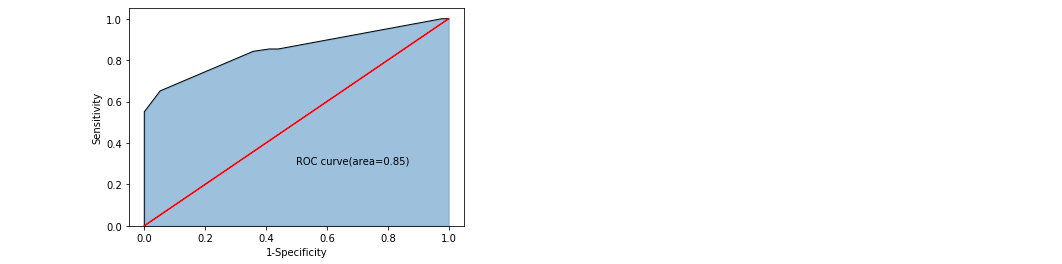

To build a random forest model:

#Building random forest can improve the prediction accuracy of a single decision tree
from sklearn import ensemble

RF_class=ensemble.RandomForestClassifier(n_estimators=200,random_state=1234)

#Fitting of random forest
RF_class.fit(X_train,y_train)

#Prediction of model on test set
RFclass_pred=RF_class.predict(X_test)

#Accuracy of the model
print('The prediction accuracy of the model in the test set is:',metrics.accuracy_score(y_test,RFclass_pred))

The accuracy of random forest is 0.85, which is higher than that of single decision tree.
Draw a picture to see the accuracy:

#Calculate plot data
y_score=RF_class.predict_proba(X_test)[:,1]
fpr,tpr,threshold=metrics.roc_curve(y_test,y_score)

#Calculate AUC value
roc_auc=metrics.auc(fpr,tpr)

#Draw area map
plt.stackplot(fpr,tpr,color='steelblue',alpha=0.5,edgecolor='black')

#Add marginal line
plt.plot(fpr,tpr,color='black',lw=1)

#Add diagonal
plt.plot([0,1],[0,1],color='red',linestyle='-')

#Add text message
plt.text(0.5,0.3,'ROC curve(area=%0.2f)'%roc_auc)

#Add x and y labels
plt.xlabel('1-Specificity')
plt.ylabel('Sensitivity')

#display graphics
plt.show()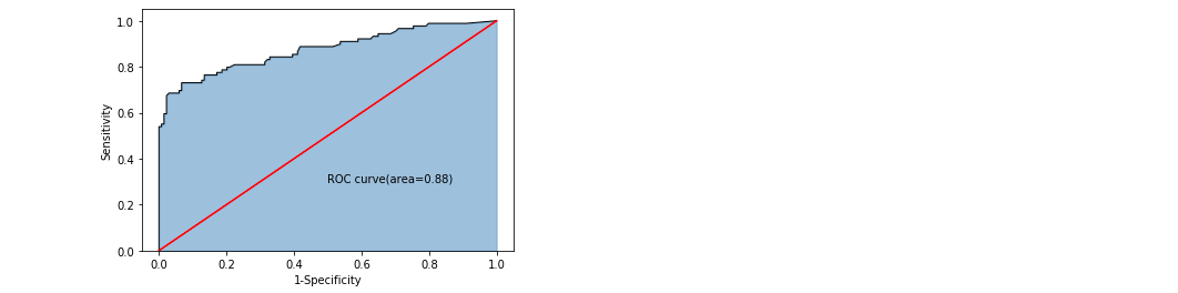

What factors determine the rescue rate on the Titanic

#Importance of independent variable
importance=RF_class.feature_importances_

#Build sequence for drawing
Impt_Series=pd.Series(importance,index=X_train.columns)

#Sort plots on a sequence
Impt_Series.sort_values(ascending=True).plot(kind='barh')
plt.show()

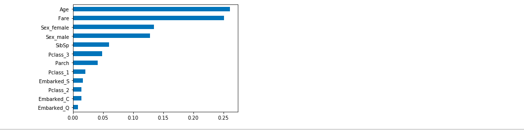
The conclusion is obvious. Do you have any inspiration?