Decision tree is a basic classification and regression method
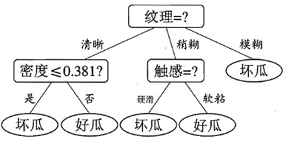
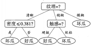
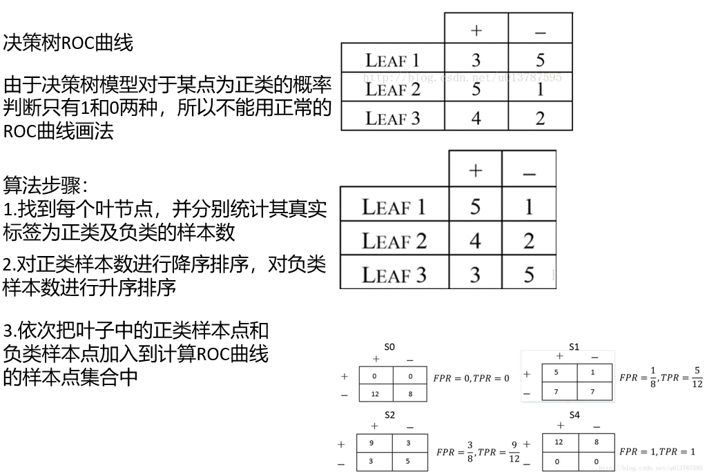
1, Basic concepts of decision tree
- The nodes and directed edges of the decision tree are represented respectively:
- An internal node represents a feature or attribute
- Leaf nodes represent a classification.
- A directed edge represents a partition rule
-
The directed edge of the decision tree from the root node to the child node represents a path
-
The paths of the decision tree are mutually exclusive and complete
-
When using decision tree classification, it is to test a feature of the sample and allocate the sample according to the test results. If the sample is allocated to the child nodes of the tree, each child node should take a value of the feature
-
Advantages of decision tree: strong readability and fast classification speed
The decision tree follows the idea of divide and rule and can be considered as a set of if else then rules
2, Decision tree algorithm index
1. Information entropy / purity
Information entropy is used to measure uncertainty. The greater the entropy, the greater the uncertainty of information
For the classification problem, the greater the entropy of the current category, the greater its uncertainty, the worse the classification effect, and the impure the set
H
(
D
)
=
E
n
t
(
D
)
=
∑
i
=
1
n
−
p
i
log
2
p
i
H\left( D \right) =Ent\left( D \right) =\sum_{i=1}^n{-p_i\log _2p_i}
H(D)=Ent(D)=i=1∑n−pilog2pi
(
n
n
n is the number of classifications,
p
i
p_i
pi (is the probability of occurrence of the current classification)
The information entropy is 0, which means that the information is determined and the classification is completed
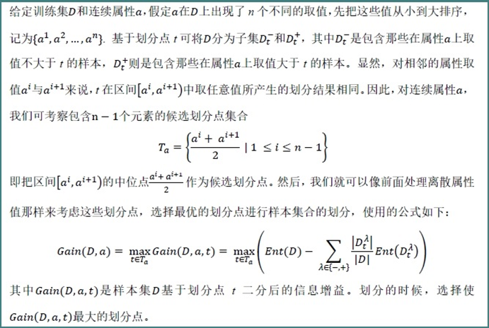
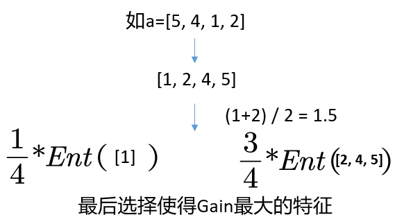
2. Information gain
If the discrete attribute A has V possible values and is divided by A against D, it will have A weight of
∣
D
v
∣
∣
D
∣
\frac{|D^v|}{|D|}
For the branch node of ∣ D ∣ Dv ∣, the increased entropy is Information Gain:
G
a
i
n
(
D
,
A
)
=
E
n
t
(
D
)
−
∑
v
=
1
V
∣
D
v
∣
∣
D
∣
E
n
t
(
D
v
)
Gain\left( D,A \right) =Ent\left( D \right) -\sum_{v=1}^V{\frac{|D^v|}{|D|}Ent\left( D^v \right)}
Gain(D,A)=Ent(D)−∑v=1V∣D∣∣Dv∣Ent(Dv)
The greater the information gain, the greater the improvement of set purity obtained by dividing with attribute A
3.ID3
ID3 (iterative dichotomizor 3) iterates the second classification and the third generation, selects the features with the information gain criterion, determines the performance of the classifier, and constructs the decision tree
Algorithm idea: using data annotation, information gain and traversal, we can complete the selection of features and thresholds in a decision tree (get the features and thresholds with the maximum information gain) and get a classification decision tree
4. Information gain rate, ID4 5 and Gini index
The information gain criterion has a preference for features with a large number of values. In order to reduce the possible adverse effects of this preference, C4 5 decision tree algorithm uses "gain rate"
G
a
i
n
_
r
a
t
i
o
(
D
,
a
)
=
G
a
i
n
(
D
,
a
)
I
V
(
a
)
Gain\_ratio\left( D,a \right) =\frac{Gain\left( D,a \right)}{IV\left( a \right)}
Gain_ratio(D,a)=IV(a)Gain(D,a)
I
V
(
a
)
=
−
∑
v
=
1
V
∣
D
v
∣
∣
D
∣
log
2
∣
D
v
∣
∣
D
∣
IV\left( a \right) =-\sum_{v=1}^V{\frac{|D^v|}{|D|}}\log _2\frac{|D^v|}{|D|}
IV(a)=−∑v=1V∣D∣∣Dv∣log2∣D∣∣Dv∣
Where IV(a) is called the intrinsic value of a, that is, the more desirable values of a, the greater IV(a)
The purity of data set D can be measured by Gini index:
G
i
n
i
(
D
)
=
∑
k
=
1
∣
y
∣
∑
k
'
≠
k
p
k
p
k
'
=
1
−
∑
k
=
1
∣
y
∣
p
k
2
Gini\left( D \right) =\sum_{k=1}^{|y|}{\sum_{k^'\ne k}{p_kp_{k^'}}}=1-\sum_{k=1}^{|y|}{p_{k}^{2}}
Gini(D)=∑k=1∣y∣∑k'=kpkpk'=1−∑k=1∣y∣pk2
The smaller Gini(D), the higher the purity of D
3, Decision tree algorithm
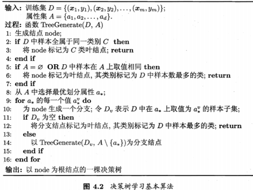
The algorithm of decision tree learning is usually to traverse, select the optimal feature and eigenvalue, and segment the training data according to the feature, so that each sub data set has the best classification. This process corresponds to the division of feature space and the construction of decision tree.
Optimal feature selection:
1. Discrete features: directly calculate the features corresponding to the maximum information gain according to the information gain formula
2. Continuous features: adopt continuous feature discretization technology and use dichotomy to process continuous features
The tree building process is recursive. There are three recursive return conditions:
1. Samples in D belong to the same category
2. D is an empty set and cannot be divided
3. The sample in D has the same value on all attributes or the attribute set is empty
4, ROC curve of decision tree
5, Implementation of continuous valued decision tree
import numpy as np
import math
from matplotlib import pyplot as plt


def loadDataSet(trainfile):  # Load data
    dataMat = []
    lable = []
    lablename = ['A', 'B', 'C', 'D', 'E', 'F', 'G', 'H']
    fr = open(trainfile)
    for line in fr.readlines():
        lineArr = line.strip().split(',')
        dataMat.append([float(lineArr[1]), float(lineArr[2]), float(lineArr[3]), float(lineArr[4]), float(lineArr[5]),
                        float(lineArr[6]), float(lineArr[7]), float(lineArr[8])])
        lable.append(float(lineArr[0]))
    return dataMat, lable, lablename


def splitdata0(dataset, lable, lable_position, best_t):  # Separate the data set excluding A attribute according to the best partition point of A: smaller than the partition point
    splitDataSet = []
    splitlable = []
    for i in range(len(dataset)):
        if dataset[i][lable_position] <= best_t:
            DataSet = dataset[i][:lable_position]  # Label will not be included_ Point at position
            DataSet.extend(dataset[i][lable_position + 1:])
            splitDataSet.append(DataSet)
            splitlable.append(lable[i])
    return splitDataSet, splitlable


def splitdata1(dataset, lable, lable_position, best_t):  # Separate the data set after eliminating the A attribute according to the best partition point of A: larger than the partition point
    splitDataSet = []
    splitlable = []
    for i in range(len(dataset)):
        if dataset[i][lable_position] > best_t:
            DataSet = dataset[i][:lable_position]  # Label will not be included_ Point at position
            DataSet.extend(dataset[i][lable_position + 1:])
            splitDataSet.append(DataSet)
            splitlable.append(lable[i])
    return splitDataSet, splitlable


def Ent(pt, pf):  # Calculate the information entropy. pt is a positive example and pf is a negative example
    if pt == 0 or pf == 0:
        return 0
    else:
        return -pt / (pt + pf) * math.log(pt / (pt + pf)) - pf / (pt + pf) * math.log(pf / (pt + pf), 2)


def Gain(A, lable):  # Information gain; Attributes; Continuous value processing
    A = np.asarray(A)
    lable = np.asarray(lable)
    T = []
    t_star, max_gain = 0.0, 0.0  # Optimal partition, middle site, maximum information gain
    pt = np.shape(np.nonzero(lable))[1]
    pf = np.shape(lable)[0] - pt
    B = np.sort(A)  # In order to get the middle site, the original list A has also changed because asarray is used
    for i in range(np.shape(B)[0] - 1):
        T.append(float((B[i] + B[i + 1]) / 2))
    m = len(T)
    for i in range(m):
        p0_t = np.shape(np.nonzero(lable[np.nonzero(A <= T[i])[0]]))[
            1]  # Number of positive examples less than or equal to T[i], NP Nonzero (a < = T[i]) [0]: index less than or equal to T[i]
        p0_f = np.shape(np.nonzero(lable[np.nonzero(A <= T[i])[0]] == 0))[1]
        p1_t = np.shape(np.nonzero(lable[np.nonzero(A > T[i])[0]]))[1]
        p1_f = np.shape(np.nonzero(lable[np.nonzero(A > T[i])[0]] == 0))[1]
        gain = Ent(pt, +pf) - ((i + 1) / m * Ent(p0_t, p0_f)) - ((m - i - 1) / m * Ent(p1_t, p1_f))
        if max_gain < gain:
            max_gain = gain
            t_star = T[i]
    return t_star, max_gain


def bestAttributes(dataSet, lable, lablename):  # Select the optimal attribute, optimal partition point and corresponding sequence number
    dataSet = np.asarray(dataSet)
    lable = np.asarray(lable)
    best_gain, best_t, best_lable, lable_position = 0.0, 0.0, 'A', 0.0
    m = np.shape(dataSet)[1]
    if len(lablename) < m:  # There are not enough attributes to select, m is the actual number of attributes
        return best_lable, best_t, lable_position
    for i in range(m):
        t, max_gain = Gain(dataSet[:, i], lable)
        if best_gain < max_gain:
            best_gain = max_gain
            best_t = t
            best_lable = lablename[i]
            lable_position = i
    return best_lable, best_t, int(lable_position)


def MostLable(lable):  # Majority vote
    lable = np.asarray(lable)
    pt = np.count_nonzero(lable)  # Count the quantity with label 1
    pf = np.shape(lable)[0] - pt
    if pt > pf:
        return 1
    else:
        return 0


def TreeGenerate(dataSet, lable, lablename):  # Spanning tree
    if len(set(lable)) == 1:  # All sample categories are consistent
        return lable[0]
    if len(dataSet[0]) == 0:  # All properties are divided, that is, the number of columns is 0
        return MostLable(lable)
    best_lable, best_t, lable_position = bestAttributes(dataSet, lable, lablename)  # The optimal label, optimal partition point and sequence number of optimal partition point are obtained
    if best_t == 0:  # Samples have the same value on a certain attribute
        return MostLable(lable)
    tree = {best_lable: {}}
    del (lablename[lable_position])
    dataSet0, lable0 = splitdata0(dataSet, lable, lable_position, best_t)
    dataSet1, lable1 = splitdata1(dataSet, lable, lable_position, best_t)
    tree[best_lable]['<=' + str(round(best_t, 3))] = TreeGenerate(dataSet0, lable0, lablename)
    tree[best_lable]['>' + str(round(best_t, 3))] = TreeGenerate(dataSet1, lable1, lablename)
    return tree


def predict(tree, feat, data, T, leaf, y, inde):
    firstFeat = list(tree.keys())[0]  # Root node properties
    secondDict = tree[firstFeat]  # Subtree of root node
    featIndex = feat.index(firstFeat)  # The sequence number (number) of firstFeat in feat, that is, which attribute corresponds!!!!!!
    for key in secondDict.keys():  # There are < = and > key s
        if data[featIndex] <= T[featIndex]:  # Since the attribute order of data is ABCDEFGH, ABCDEFGH should also be used in T, otherwise an error will occur
            ture_key = '<=' + str(T[featIndex])
            if ture_key == key:  # String equality
                if type(secondDict[key]).__name__ == "dict":  # If the child node is a dictionary type, it recurses until it is a number
                    classlable = predict(secondDict[key], feat, data, T, leaf, y, inde)
                else:
                    classlable = secondDict[key]
                    if str(key[2:7]) == '0.151':
                        if y[inde] == 0:
                            leaf[str(key[2:7]) + '0' + '0'] += 1
                        else:
                            leaf[str(key[2:7]) + '0' + '1'] += 1
                    else:
                        if y[inde] == 0:
                            leaf[str(key[2:7]) + '0'] += 1
                        else:
                            leaf[str(key[2:7]) + '1'] += 1
        else:
            ture_key = '>' + str(T[featIndex])
            if ture_key == key:
                if type(secondDict[key]).__name__ == "dict":
                    classlable = predict(secondDict[key], feat, data, T, leaf, y, inde)
                else:
                    classlable = secondDict[key]
                    if str(key[1:6]) == '0.151':
                        if y[inde] == 0:
                            leaf[str(key[1:6]) + '1' + '0'] += 1
                        else:
                            leaf[str(key[1:6]) + '1' + '1'] += 1
                    else:
                        if y[inde] == 0:
                            leaf[str(key[1:6]) + '0'] += 1
                        else:
                            leaf[str(key[1:6]) + '1'] += 1
    return classlable


def getKey(x):
    return float(x[0])


def roc_draw(leaf):
    mat = np.zeros((9, 2))
    i = j = 0
    sum1 = sum0 = 0
    for key, value in leaf.items():
        if key[-1] == '0':
            mat[i][1] = value
            sum0 += value
            i += 1
        else:
            mat[j][0] = value
            sum1 += value
            j += 1
    col_one = mat[:, 0]
    col_two = mat[:, 1]
    col_one = np.sort(col_one)
    col_two = np.sort(col_two)
    mat = np.vstack((col_one, col_two)).T
    fpr = [0]
    tpr = [0]
    s0 = s1 = 0
    s = 0
    for i, j in mat:
        print(j, i)
        temp0 = s0
        temp1 = s1
        s1 += i
        s0 += j
        s += (((temp1 + s1) / sum1) * (j / sum0) / 2)
        fpr.append(s0 / sum0)
        tpr.append(s1 / sum1)
    plt.plot(fpr, tpr, color='red')
    plt.xlabel("False Positive Rate(FPR)")
    plt.ylabel("Ture Positive Rate(TPR)")
    plt.grid(alpha=0.4)
    plt.show()
    return s


def con_mat(true_lable, pre_lable):
    tp, fp, fn, tn = 0, 0, 0, 0
    for i in range(len(true_lable)):
        if true_lable[i] == pre_lable[i]:
            if true_lable[i] == 1:
                tp += 1
            else:
                tn += 1
        else:
            if true_lable[i] == 1:
                fn += 1
            else:
                fp += 1

    print("confusion matrix:", tp, fp)
    print("                 ", fn, tn)
    print("accuracy:        ", (tp + tn) / (tp + tn + fn + fp))
    print("precisionScore:  ", tp / (tp + fp))
    print("recallScore:     ", tp / (tp + fn))
    print("F1:              ", tp / (tp + (fn + fp) / 2))
    return


traindata, trainlable, lablename = loadDataSet('classification_train.txt')
tree = TreeGenerate(traindata, trainlable, lablename)
print(tree)

# verification
testdata, testlable, testlablename = loadDataSet('classification_test.txt')
T = [0.235, 0.617, 0.607, 0.165, 0.151, 0.446, 0.036, 0.008]
pre_lable = []
feat = ['A', 'B', 'C', 'D', 'E', 'F', 'G', 'H']

leaf = {}
leaf['0.2350'] = leaf['0.6170'] = leaf['0.6070'] = leaf['0.1650'] = leaf['0.4460'] = leaf['0.0360'] = \
    leaf['0.0080'] = 0
leaf['0.2351'] = leaf['0.6171'] = leaf['0.6071'] = leaf['0.1651'] = leaf['0.4461'] = leaf['0.0361'] = \
    leaf['0.0081'] = 0
leaf['0.15100'] = leaf['0.15101'] = leaf['0.15110'] = leaf['0.15111'] = 0
inde = 0
for data in testdata:
    pre_lable.append(predict(tree, feat, data, T, leaf, testlable, inde))
    inde += 1

con_mat(testlable, pre_lable)
print("ROC AUC: ", roc_draw(leaf))