1, Introduction
1.1 concept
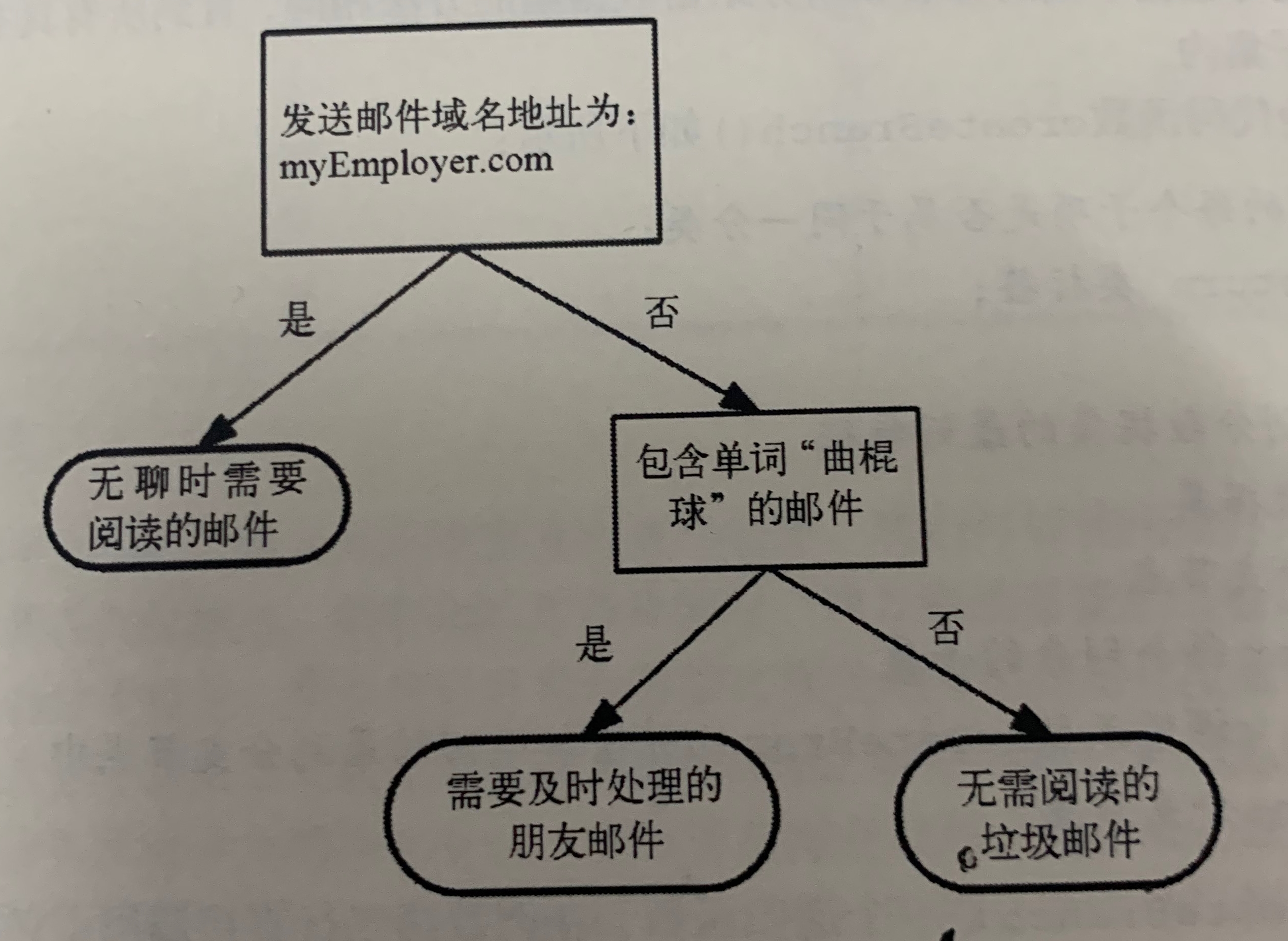
As shown in the figure, it is a decision tree. The square represents the decision block and the ellipse represents the terminating block, indicating that the conclusion has been reached and the operation can be terminated. The left and right arrow branch es are led out from the judgment module, which can reach the next judgment module or terminate the module. A hypothetical e-mail classification system is constructed.
1.2 construction of decision tree
1.2.1 general process:
1. Collect data
2. Prepare data
3. Analysis data
4. Training algorithm
5. Test algorithm
6. Use algorithm
The pseudo code function createBranch to create a branch is as follows:
Detect whether each sub item in the dataset belongs to the same classification
If so return Class label
Else
	Find the best features to divide the dataset
	Partition dataset
	Create branch node
		for Subset of each partition
			Call function createBranch And add the returned result to the branch node
	return Branch node
1.3 information gain
The change of information before and after dividing the data set is called information gain. Knowing how to calculate the information gain, we can calculate the learning gain obtained by dividing the data set by each eigenvalue. The feature with the highest information gain is the best choice.

Where n is the number of classifications
Code part for calculating Shannon entropy for a given dataset:
from math import log
import operator
def calcshannonEnt(dataSet):
    nuMEntries = len(dataSet)
    labelCounts = {}
    for featVec in dataSet:
        currentLabel = featVec[-1]
        if currentLabel not in labelCounts.keys():
            labelCounts[currentLabel] = 0
        labelCounts[currentLabel] += 1
    shannonEnt = 0.0
    for key in labelCounts:
        prob = float(labelCounts[key])/nuMEntries
        shannonEnt -= prob * log(prob,2)
    return shannonEnt
First, we need to calculate the total number of instances in the dataset. Here, we explicitly declare a variable to save the total number of instances. Then create a data dictionary whose key value is the value of the last column. If the current key value does not exist, expand the dictionary and add the current key value to the dictionary. Here, each key value records the occurrence times of the current category. Finally, the occurrence probability of all class labels is used to calculate the occurrence probability of the category. We will use this probability to calculate Shannon entropy and count the times of all class labels. Finally, the occurrence frequency of all class labels is used to calculate the probability of class occurrence.
You can use createDataSet() to get a simple authentication dataset
def createDataset():
    dataSet = [[1,1,'yes'],[1,1,'yes'],[1,0,'no'],[0,1,'no'],[0,1,'no']]
    labels = ['no surfacing','flippers']
    return dataSet,labels
The higher the entropy, the more mixed data. We can add more categories in the data set to observe how the entropy changes. We add a third category called may to test the change of entropy:
myData[0][-1]='maybe'
    print(myData)
    print(calcshannonEnt(myData))
1.4 data division
In addition to measuring the information entropy, the classification algorithm also needs to divide the data set and measure the entropy of the divided data set, so as to judge whether the data set is divided correctly. The information entropy is calculated once for the result of dividing the data set according to each feature, and then it is judged which feature is the best way to divide the data set.
Given feature Division:
def splitDataSet(dataSet, axis, value):
    # Create a list of returned datasets
    retDataSet = []
    # Traversal dataset
    for featVec in dataSet:
        if featVec[axis] == value:
            # Remove axis feature
            reducedFeatVec = featVec[:axis]
            # Add eligible to the returned dataset
            reducedFeatVec.extend(featVec[axis + 1:])
            retDataSet.append(reducedFeatVec)
    # Returns the partitioned dataset
    return retDataSet


def createDataSet():
    # data set
    dataSet = [[1, 1, 'yes'],
               [1, 1, 'yes'],
               [1, 0, 'no'],
               [0, 1, 'no'],
               [0, 1, 'no']]
    # Classification properties
    labels = ['no surfacing', 'flippers']
    # Return dataset and classification properties
    return dataSet, labels


if __name__ == '__main__':
    dataSet, labels = createDataSet()
    print(dataSet)
    print(splitDataSet(dataSet, 0, 1))
    print(splitDataSet(dataSet, 0, 0))
Select the best way to divide the data:
from math import log
def calcShannonEnt(dataSet):
# Returns the number of rows in the dataset
numEntries = len(dataSet)
# Save a dictionary of the number of occurrences of each label
labelCounts = {}
# Each group of eigenvectors is counted
for featVec in dataSet:
# Extract label information
currentLabel = featVec[-1]
# If the label is not put into the dictionary of statistical times, add it
if currentLabel not in labelCounts.keys():
labelCounts[currentLabel] = 0
# Label count
labelCounts[currentLabel] += 1
# Shannon entropy
shannonEnt = 0.0
# Calculate Shannon entropy
for key in labelCounts:
# The probability of selecting the label
prob = float(labelCounts[key])/numEntries
# Calculation of Shannon entropy by formula
shannonEnt -= prob * log(prob, 2)
# Return Shannon entropy
return shannonEnt
def splitDataSet(dataSet, axis, value):
# Create a list of returned datasets
retDataSet = []
# Traversal dataset
for featVec in dataSet:
if featVec[axis] == value:
# Remove axis feature
reducedFeatVec = featVec[:axis]
# Add eligible to the returned dataset
reducedFeatVec.extend(featVec[axis + 1:])
retDataSet.append(reducedFeatVec)
# Returns the partitioned dataset
return retDataSet
def chooseBestFeatureToSplit(dataSet):
# Number of features
numFeatures = len(dataSet[0]) - 1
# Calculate Shannon entropy of data set
baseEntropy = calcShannonEnt(dataSet)
# information gain
bestInfoGain = 0.0
# Index value of optimal feature
bestFeature = -1
# Traverse all features
for i in range(numFeatures):
# Get the i th all features of dataSet
featList = [example[i] for example in dataSet]
# Create set set {}, elements cannot be repeated
uniqueVals = set(featList)
# Empirical conditional entropy
newEntropy = 0.0
# Calculate information gain
for value in uniqueVals:
# The subset of the subDataSet after partition
subDataSet = splitDataSet(dataSet, i, value)
# Calculate the probability of subsets
prob = len(subDataSet) / float(len(dataSet))
# The empirical conditional entropy is calculated according to the formula
newEntropy += prob * calcShannonEnt(subDataSet)
# information gain
infoGain = baseEntropy - newEntropy
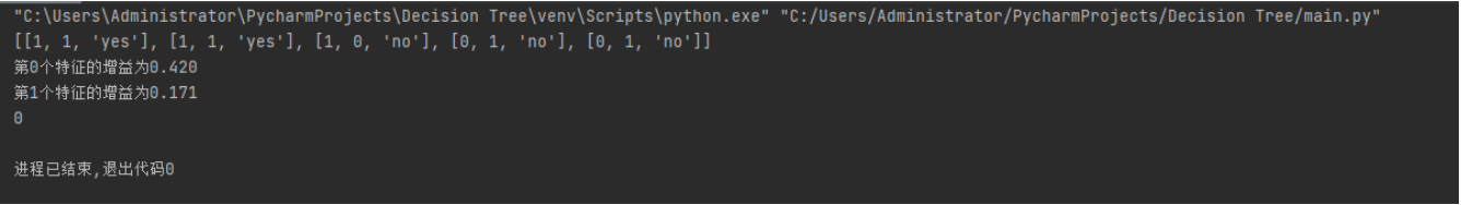
# Print information gain for each feature
print("The first%d The gain of each feature is%.3f" % (i, infoGain))
# Calculate information gain
if (infoGain > bestInfoGain):
# Update the information gain to find the maximum information gain
bestInfoGain = infoGain
# Record the index value of the feature with the largest information gain
bestFeature = i
# Returns the index value of the feature with the largest information gain
return bestFeature
Operation screenshot:
1.5 recursive construction of decision tree
Working principle: get the original data set, and then divide the data set based on the best attribute value. Since there may be more than two eigenvalues, there may be data set division greater than two branches. After the first division, the data will be passed down to the next node of the tree branch. On this node, we can divide the data again, Therefore, we can use the principle of recursion to deal with data sets.
Conditions for the end of recursion: the program traverses the attributes of all partitioned data sets, or all instances under each branch have the same classification. If all instances have the same classification, a leaf node or termination block is obtained, and any data reaching the leaf node must belong to the classification of the leaf node.
If the class label is still not unique after the dataset has processed all attributes, we need to decide how to define the leaf node. We usually use the majority voting method to determine the classification of the leaf node. The code is as follows:
def majorityCnt(classList):
    classCount={}
    for vote in classList: #Count the number of occurrences of each element in the classList
        if vote not in classCount.keys():classCount[vote]=0
        classCount[vote]+=1
    sortedClassCount=sorted(classCount.iteritems(),key=operator.itemgetter(1),reverse=True) #Sort dictionary
    return sortedClassCount[0][0]
The code for creating the tree is as follows:
def createTree(dataSet,labels):
    classList = [example[-1] for example in dataSet]
    if classList.count(classList[0]) == len(classList):#If the categories are exactly the same, continue to divide
        return classList[0]
    if len(dataSet[0]) == 1: #When all features are traversed, the category with the most occurrences is returned
        return majorityCnt(classList)
    bestFeat = chooseBestFeatureTOSplit(dataSet) #Select the optimal feature
    bestFeatLabel = labels[bestFeat] #Optimal feature label
    myTree = {bestFeatLabel:{}}
    del (labels[bestFeat]) #Get all attribute values contained in the list
    featValues = [example[bestFeat] for example in dataSet]
    uniqueVals = set(featValues)
    for value in uniqueVals: #Create decision tree
        subLabels = labels[:]
        myTree[bestFeatLabel][value] = createTree(splitDataSet(dataSet,bestFeat,value),subLabels)
    return myTree
The variable myTree contains many nested dictionaries representing tree structure information. Starting from the left, the first keyword no surfacing is the feature name of the first partitioned dataset, and the value of this keyword is another data dictionary. The second keyword is the data set divided by the no surfacing feature. The values of these keywords are the child nodes of the no surfacing node. These values may be class labels or another data dictionary. If the value is a class label, the child node is a leaf node; If the value is another data dictionary, the child node is a judgment node. This format structure repeats continuously to form the whole tree. This tree contains three leaf nodes and two judgment nodes.
2, Drawing a tree in python using the Matplotlib annotation
Draw tree nodes with text annotations:
import matplotlib.pyplot as plt
from pylab import mpl
decisionNode = dict(boxstyle='sawtooth',fc="0.8")#Define text box and arrow formats
leafNode = dict(boxstyle="round4",fc="0.8")
arrow_args = dict(arrowstyle="<-")
def plotNode(nodeTxt,centerPt,parentPt,nodeType):#Draw annotation with arrow
    createPlot.ax1.annotate(nodeTxt,xy=parentPt,xycoords='axes fraction',xytext=centerPt,textcoords='axes fraction',va="center",ha="center",bbox=nodeType,arrowprops=arrow_args)
def createPlot():
    fig = plt.figure(1,facecolor='white')
    fig.clf()
    createPlot.ax1 = plt.subplot(111,frameon=False)
    mpl.rcParams['font.sans-serif'] = ['SimHei']  # Blackbody
    plotNode('Decision node',(0.5,0.1),(0.1,0.5),decisionNode)
    plotNode('Leaf node',(0.8,0.1),(0.3,0.8),leafNode)
    plt.show()
Operation screenshot:

I haven't finished it yet. I'll write it tomorrow. 55555!!!!