Author: baiyucraft

BLog: baiyucraft's Home

Original text: Hands on learning and deep learning

1, Differential and derivative

   I believe everyone knows the concept. Draw a picture according to the book:

import numpy as np
from matplotlib import pyplot as plt


def set_figsize(figsize=(3.5, 2.5)):
    """set up matplotlib The size of the chart."""
    plt.rcParams['figure.figsize'] = figsize


def set_axes(axes, xlabel, ylabel, xlim, ylim, xscale, yscale, legend):
    """set up matplotlib The axis of the."""
    axes.set_xlabel(xlabel)
    axes.set_ylabel(ylabel)
    axes.set_xscale(xscale)
    axes.set_yscale(yscale)
    axes.set_xlim(xlim)
    axes.set_ylim(ylim)
    if legend:
        axes.legend(legend)
    axes.grid()


def plot(X, Y=None, xlabel=None, ylabel=None, legend=None, xlim=None, ylim=None, xscale='linear', yscale='linear',
         fmts=('-', 'm--', 'g-.', 'r:'), axes=None):
    """Draw data points."""
    if legend is None:
        legend = []

    # Set canvas size
    set_figsize((4, 2.5))
    # Move axis
    axes = axes if axes else plt.gca()

    # If 'X' has an axis, output True
    def has_one_axis(X):
        return hasattr(X, "ndim") and X.ndim == 1 or isinstance(X, list) and not hasattr(X[0], "__len__")

    if has_one_axis(X):
        X = [X]
    if not Y:
        X, Y = [[]] * len(X), X
    elif has_one_axis(Y):
        Y = [Y]
    if len(X) != len(Y):
        X = X * len(Y)
    # Clears the currently active axis
    axes.cla()
    for x, y, fmt in zip(X, Y, fmts):
        if len(x):
            axes.plot(x, y, fmt)
        else:
            axes.plot(y, fmt)
    set_axes(axes, xlabel, ylabel, xlim, ylim, xscale, yscale, legend)
    plt.show()


if __name__ == '__main__':
    def f(x):
        return 3 * x ** 2 - 4 * x
    
    def g(x):
        return 2 * x - 3

    x = np.arange(0, 3, 0.1)
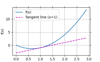
    plot(x, [f(x), g(x)], 'x', 'f(x)', legend=['f(x)', 'Tangent line (x=1)'])

Operation results:

2, Automatic derivation

   pytorch can calculate the derivative by automatic derivation. In practice, according to the model we designed, the system will build a calculation diagram to track which data is calculated and which operations are combined to produce output. Automatic derivation enables the system to subsequently back propagate the gradient. So the back-propagation function used in derivation

1. Derivation of scalar vector

We want to do a function y = 2 x T x y = 2x^{T}x y=2xTx about column vector x x x derivative:

x = torch.arange(4.0)
# Can store gradient
x.requires_grad_(True)
print('\n======x======\n', x)
# y = 2x^{T}x
y = 2 * torch.dot(x, x)
print('\n======y======\n', y)
# Call back propagation function
# y = 2x1**2 + 2x2**2 + 2x3**2 + 2x4**2 after derivation, 4 * (x1, x2, x3, x4)
y.backward()
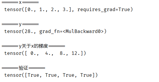
print('\n======y about x Gradient of======\n', x.grad)
print('\n======verification======\n', x.grad == 4 * x)

Operation results:

  now let's calculate x x Another function of x:

# By default, PyTorch will accumulate gradients, and we need to clear the previous value
x.grad.zero_()
y = x.sum()
print('\n======x======\n', x)
print('\n======y======\n', y)
y.backward()
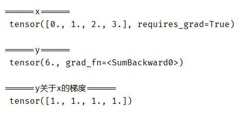
print('\n======y about x Gradient of======\n', x.grad)

Operation results:

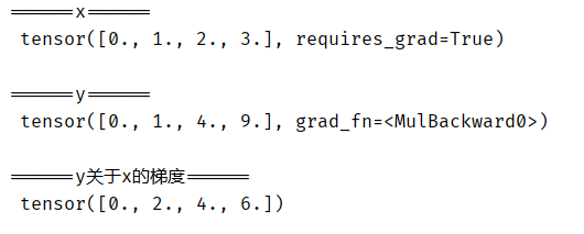
2. Back propagation of non scalar variables

   when y is not a scalar, the most natural explanation for the derivative of vector y with respect to vector x is a matrix. For higher-order tensors, the sum of derivatives of y can be a result of higher-order tensors.

  however, although these more exotic objects do appear in advanced machine learning (including deep learning), when we call the inverse calculation of vectors, we usually try to calculate the derivative of the loss function of each component in a batch of training samples. Here, our purpose is not to calculate the differential matrix, but the sum of the partial derivatives calculated separately for each sample in the batch.

# Calling 'backward' for non scalar needs to pass in a 'gradient' parameter, which specifies the gradient of the differential function about 'self'. In our example, we just want to sum the partial derivatives, so it's appropriate to pass a gradient of 1
x.grad.zero_()
y = x * x
print('\n======x======\n', x)
print('\n======y======\n', y)
# Equivalent to y.backward(torch.ones(len(x)))
y.sum().backward()
print('\n======y about x Gradient of======\n', x.grad)

Operation results:

3. Separation calculation

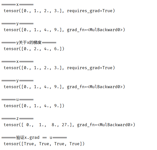
  sometimes we want to move some calculations out of the recorded calculation diagram. For some reason, we want to treat y as a constant and only consider the role of x after y is calculated. Here, we can use the detach() function to change y into a constant u relative to x:

# Separation calculation
x.grad.zero_()
y = x * x
print('\n======x======\n', x)
print('\n======y======\n', y)
u = y.detach()
print('\n======u======\n', u)
z = u * x
print('\n======z======\n', z)
z.sum().backward()
print('\n======verification x.grad == u======\n', x.grad == u)

Operation results:

4. Gradient calculation of Python control flow

   one advantage of using automatic derivation is that we can still calculate the gradient of the variable even if the calculation diagram of the function needs to be controlled by Python (for example, condition, loop or arbitrary function call). In the following code, the number of iterations of the while loop and the result of the if statement depend on the value of input a:

# Gradient calculation of Python control flow
def f(a):
    b = a * 2
    while b.norm() < 1000:
        b = b * 2
    if b.sum() > 0:
        c = b
	else:
        c = 100 * b
	return c

a = torch.randn(size=(), requires_grad=True)
d = f(a)
d.backward()
print('\n======a======\n', a)
print('\n======f(a)======\n', d)
print('\n======f(a)about a Gradient of======\n', a.grad)
print('\n======verification======\n', a.grad == d / a)

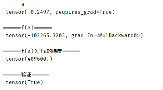
Operation results: